Tutorial: Linear Programming, (CPLEX Part 1)
This notebook gives an overview of Linear Programming (or LP). After completing this unit, you should be able to
- describe the characteristics of an LP in terms of the objective, decision variables and constraints,
- formulate a simple LP model on paper,
- conceptually explain some standard terms related to LP, such as dual, feasible region, infeasible, unbounded, slack, reduced cost, and degenerate.
You should also be able to describe some of the algorithms used to solve LPs, explain what presolve does, and recognize the elements of an LP in a basic DOcplex model.
This notebook is part of Prescriptive Analytics for Python
It requires either an installation of CPLEX Optimizers or it can be run on IBM Cloud Pak for Data as a Service (Sign up for a free IBM Cloud account and you can start using
IBM Cloud Pak for Data as a Serviceright away).CPLEX is available on IBM Cloud Pack for Data and IBM Cloud Pak for Data as a Service:
- IBM Cloud Pak for Data as a Service: Depends on the runtime used:
- Python 3.x runtime: Community edition
- Python 3.x + DO runtime: full edition
- Cloud Pack for Data: Community edition is installed by default. Please install the
DOaddon inWatson Studio Premiumfor the full edition
Table of contents:
Introduction to Linear Programming
In this topic, you’ll learn what the basic characteristics of a linear program are.
What is Linear Programming?
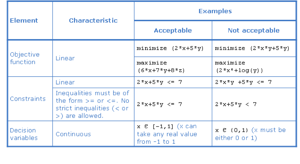
Linear programming deals with the maximization (or minimization) of a linear objective function, subject to linear constraints, where all the decision variables are continuous. That is, no discrete variables are allowed. The linear objective and constraints must consist of linear expressions.
What is a linear expression?
A linear expression is a scalar product, for example, the expression:
$$ \sum{a_i x_i} $$where a_i represents constants (that is, data) and x_i represents variables or unknowns.
Such an expression can also be written in short form as a vector product:
$$^{t}A X $$where $A$ is the vector of constants and $X$ is the vector of variables.
Note: Nonlinear terms that involve variables (such as x and y) are not allowed in linear expressions. Terms that are not allowed in linear expressions include
- multiplication of two or more variables (such as x times y),
- quadratic and higher order terms (such as x squared or x cubed),
- exponents,
- logarithms,
- absolute values.
What is a linear constraint?
A linear constraint is expressed by an equality or inequality as follows:
- $linear\_expression = linear\_expression$
- $linear\_expression \le linear\_expression$
- $linear\_expression \ge linear\_expression$
Any linear constraint can be rewritten as one or two expressions of the type linear expression is less than or equal to zero.
Note that strict inequality operators (that is, $>$ and $<$) are not allowed in linear constraints.
What is a continuous variable?
A variable (or decision variable) is an unknown of the problem. Continuous variables are variables the set of real numbers (or an interval).
Restrictions on their values that create discontinuities, for example a restriction that a variable should take integer values, are not allowed.
Symbolic representation of an LP
A typical symbolic representation of a Linear Programming is as follows:
$ minimize \sum c_{i} x_{i}\\ \\ subject\ to:\\ \ a_{11}x_{1} + a_{12} x_{2} ... + a_{1n} x_{n} \ge b_{1}\\ \ a_{21}x_{1} + a_{22} x_{2} ... + a_{2n} x_{n} \ge b_{2}\\ ... \ a_{m1}x_{1} + a_{m2} x_{2} ... + a_{mn} x_{n} \ge b_{m}\\ x_{1}, x_{2}...x_{n} \ge 0 $
This can be written in a concise form using matrices and vectors as:
$ min\ C^{t}x\\ s.\ t.\ Ax \ge B\\ x \ge 0 $
Where $x$ denotes the vector of variables with size $n$, $A$ denotes the matrix of constraint coefficients, with $m$ rows and $n$ columns and $B$ is a vector of numbers with size $m$.
Characteristics of a linear program
Example: a production problem
In this topic, you’ll analyze a simple production problem in terms of decision variables, the objective function, and constraints.
You’ll learn how to write an LP formulation of this problem, and how to construct a graphical representation of the model. You’ll also learn what feasible, optimal, infeasible, and unbounded mean in the context of LP.
Problem description: telephone production
A telephone company produces and sells two kinds of telephones, namely desk phones and cellular phones.
Each type of phone is assembled and painted by the company. The objective is to maximize profit, and the company has to produce at least 100 of each type of phone.
There are limits in terms of the company’s production capacity, and the company has to calculate the optimal number of each type of phone to produce, while not exceeding the capacity of the plant.
Writing a descriptive model
It is good practice to start with a descriptive model before attempting to write a mathematical model. In order to come up with a descriptive model, you should consider what the decision variables, objectives, and constraints for the business problem are, and write these down in words.
In order to come up with a descriptive model, consider the following questions:
- What are the decision variables?
- What is the objective?
- What are the constraints?
Telephone production: a descriptive model
A possible descriptive model of the telephone production problem is as follows:
- Decision variables:
- Number of desk phones produced (DeskProduction)
- Number of cellular phones produced (CellProduction)
- Objective: Maximize profit
- Constraints:
- The DeskProduction should be greater than or equal to 100.
- The CellProduction should be greater than or equal to 100.
- The assembly time for DeskProduction plus the assembly time for CellProduction should not exceed 400 hours.
- The painting time for DeskProduction plus the painting time for CellProduction should not exceed 490 hours.
Writing a mathematical model
Convert the descriptive model into a mathematical model:
- Use the two decision variables DeskProduction and CellProduction
- Use the data given in the problem description (remember to convert minutes to hours where appropriate)
- Write the objective as a mathematical expression
- Write the constraints as mathematical expressions (use “=”, “<=”, or “>=”, and name the constraints to describe their purpose)
- Define the domain for the decision variables
Telephone production: a mathematical model
To express the last two constraints, we model assembly time and painting time as linear combinations of the two productions, resulting in the following mathematical model:
$ maximize:\\ \ \ 12\ desk\_production + 20\ cell\_production\\ subject\ to: \\ \ \ desk\_production >= 100 \\ \ \ cell\_production >= 100 \\ \ \ 0.2\ desk\_production + 0.4\ cell\_production <= 400 \\ \ \ 0.5\ desk\_production + 0.4\ cell\_production <= 490 \\ $
Using DOcplex to formulate the mathematical model in Python
Use the DOcplex Python library to write the mathematical model in Python. This is done in four steps:
- create a instance of docplex.mp.Model to hold all model objects
- create decision variables,
- create linear constraints,
- finally, define the objective.
But first, we have to import the class Model from the docplex module.
Use IBM Decision Optimization CPLEX Modeling for Python
Let's use the DOcplex Python library to write the mathematical model in Python.
Step 1: Download the library
Install CPLEX (Community Edition) and docplex if they are not installed.
In IBM Cloud Pak for Data as a Service notebooks, CPLEX and docplex are preinstalled.
import sys
try:
    import cplex
except:
    if hasattr(sys, 'real_prefix'):
        #we are in a virtual env.
        !pip install cplex
    else:
        !pip install --user cplex
Installs DOcplexif needed
import sys
try:
    import docplex.mp
except:
    if hasattr(sys, 'real_prefix'):
        #we are in a virtual env.
        !pip install docplex
    else:
        !pip install --user docplex
If either CPLEX or docplex where installed in the steps above, you will need to restart your jupyter kernel for the changes to be taken into account.
# first import the Model class from docplex.mp
from docplex.mp.model import Model

# create one model instance, with a name
m = Model(name='telephone_production')
Define the decision variables
- The continuous variable
deskrepresents the production of desk telephones. - The continuous variable
cellrepresents the production of cell phones.
# by default, all variables in Docplex have a lower bound of 0 and infinite upper bound
desk = m.continuous_var(name='desk')
cell = m.continuous_var(name='cell')
Set up the constraints
- Desk and cell phone must both be greater than 100
- Assembly time is limited
- Painting time is limited.
# write constraints
# constraint #1: desk production is greater than 100
m.add_constraint(desk >= 100)

# constraint #2: cell production is greater than 100
m.add_constraint(cell >= 100)

# constraint #3: assembly time limit
ct_assembly = m.add_constraint( 0.2 * desk + 0.4 * cell <= 400)

# constraint #4: paiting time limit
ct_painting = m.add_constraint( 0.5 * desk + 0.4 * cell <= 490)
Express the objective
We want to maximize the expected revenue.
m.maximize(12 * desk + 20 * cell)
A few remarks about how we formulated the mathemtical model in Python using DOcplex:
- all arithmetic operations (+, *, -) are done using Python operators
- comparison operators used in writing linear constraint use Python comparison operators too.
Print information about the model
We can print information about the model to see how many objects of each type it holds:
m.print_information()
Graphical representation of a Linear Problem
A simple 2-dimensional LP (with 2 decision variables) can be represented graphically using a x- and y-axis.
This is often done to demonstrate optimization concepts.
To do this, follow these steps:
- Assign one variable to the x-axis and the other to the y-axis.
- Draw each of the constraints as you would draw any line in 2 dimensions.
- Use the signs of the constraints (=, <= or >=) to determine which side of each line falls within the feasible region (allowable solutions).
- Draw the objective function as you would draw any line in 2 dimensions, by substituting any value for the objective (for example, 12 DeskProduction + 20 CellProduction = 4000)
Feasible set of solutions
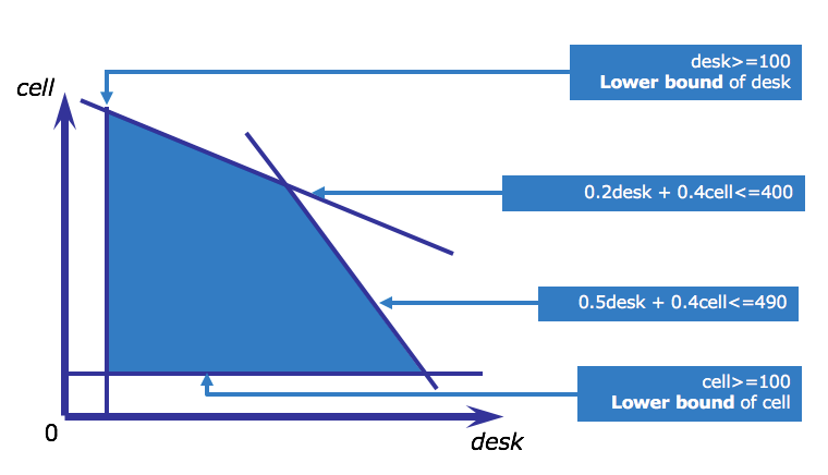
This graphic shows the feasible region for the telephone problem.
Recall that the feasible region of an LP is the region delimited by the constraints, and it represents all feasible solutions. In this graphic, the variables DeskProduction and CellProduction are abbreviated to be desk and cell instead. Look at this diagram and search intuitively for the optimal solution. That is, which combination of desk and cell phones will yield the highest profit.
The optimal solution
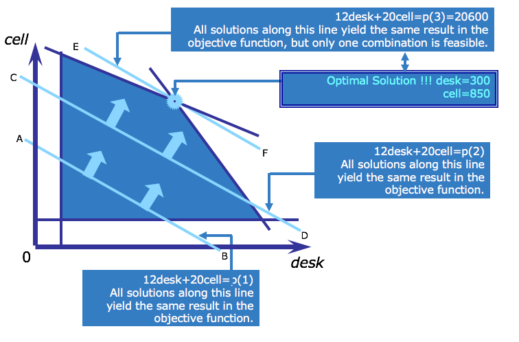
To find the optimal solution to the LP, you must find values for the decision variables, within the feasible region, that maximize profit as defined by the objective function. In this problem, the objective function is to maximize $$12 * desk + 20 * cell $$
To do this, first draw a line representing the objective by substituting a value for the objective.
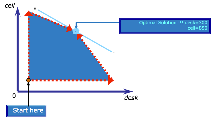
Next move the line up (because this is a maximization problem) to find the point where the line last touches the feasible region. Note that all the solutions on one objective line, such as AB, yield the same objective value. Other values of the objective will be found along parallel lines (such as line CD).
In a profit maximizing problem such as this one, these parallel lines are often called isoprofit lines, because all the points along such a line represent the same profit. In a cost minimization problem, they are known as isocost lines. Since all isoprofit lines have the same slope, you can find all other isoprofit lines by pushing the objective value further out, moving in parallel, until the isoprofit lines no longer intersect the feasible region. The last isoprofit line that touches the feasible region defines the largest (therefore maximum) possible value of the objective function. In the case of the telephone production problem, this is found along line EF.
The optimal solution of a linear program always belongs to an extreme point of the feasible region (that is, at a vertex or an edge).
Solve with the model
If you're using a Community Edition of CPLEX runtimes, depending on the size of the problem, the solve stage may fail and will need a paying subscription or product installation.
In any case, Model.solve() returns a solution object in Python, containing the optimal values of decision variables, if the solve succeeds, or else it returns None.
s = m.solve()
m.print_solution()
In this case, CPLEX has found an optimal solution at (300, 850). You can check that this point is indeed an extreme point of the feasible region.
Multiple Optimal Solutions
It is possible that an LP has multiple optimal solutions. At least one optimal solution will be at a vertex. By default, the CPLEX® Optimizer reports the first optimal solution found.
Example of multiple optimal solutions
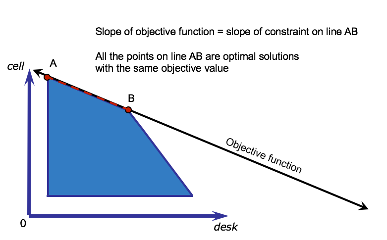
This graphic shows an example of an LP with multiple optimal solutions. This can happen when the slope of the objective function is the same as the slope of one of the constraints, in this case line AB. All the points on line AB are optimal solutions, with the same objective value, because they are all extreme points within the feasible region.
Binding and nonbinding constraints
A constraint is binding if the constraint becomes an equality when the solution values are substituted.
Graphically, binding constraints are constraints where the optimal solution lies exactly on the line representing that constraint.
In the telephone production problem, the constraint limiting time on the assembly machine is binding:
$$ 0.2desk + 0.4 cell <= 400\\ desk = 300 cell = 850 0.2(300) + 0.4(850) = 400 $$The same is true for the time limit on the painting machine:
$$ 0.5desk + 0.4cell <= 490 0.5(300) + 0.4(850) = 490 $$On the other hand, the requirement that at least 100 of each telephone type be produced is nonbinding because the left and right hand sides are not equal:
$$ desk >= 100\\ 300 \neq 100 $$Infeasibility
A model is infeasible when no solution exists that satisfies all the constraints. This may be because: The model formulation is incorrect. The data is incorrect. The model and data are correct, but represent a real-world conflict in the system being modeled.
When faced with an infeasible model, it's not always easy to identify the source of the infeasibility.
DOcplex helps you identify potential causes of infeasibilities, and it will also suggest changes to make the model feasible.
An example of infeasible problem
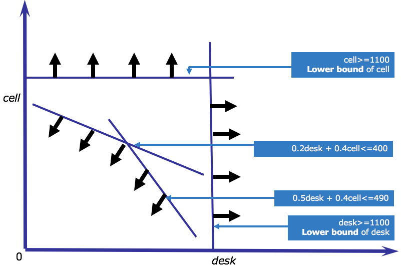
This graphic shows an example of an infeasible constraint set for the telephone production problem. Assume in this case that the person entering data had accidentally entered lower bounds on the production of 1100 instead of 100. The arrows show the direction of the feasible region with respect to each constraint. This data entry error moves the lower bounds on production higher than the upper bounds from the assembly and painting constraints, meaning that the feasible region is empty and there are no possible solutions.
Infeasible models in DOcplex
Calling solve() on an infeasible model returns None. Let's experiment this with DOcplex. First, we take a copy of our model and an extra infeasible constraint which states that desk telephone production must be greater than 1100
# create a new model, copy of m
im = m.copy()
# get the 'desk' variable of the new model from its name
idesk = im.get_var_by_name('desk')
# add a new (infeasible) constraint
im.add_constraint(idesk >= 1100);
# solve the new proble, we expect a result of None as the model is now infeasible
ims = im.solve()
if ims is None:
    print('- model is infeasible')
Correcting infeasible models
To correct an infeasible model, you must use your knowledge of the real-world situation you are modeling. If you know that the model is realizable, you can usually manually construct an example of a feasible solution and use it to determine where your model or data is incorrect. For example, the telephone production manager may input the previous month's production figures as a solution to the model and discover that they violate the erroneously entered bounds of 1100.
DOcplex can help perform infeasibility analysis, which can get very complicated in large models. In this analysis, DOcplex may suggest relaxing one or more constraints.
Relaxing constraints by changing the model
In the case of LP models, the term “relaxation” refers to changing the right hand side of the constraint to allow some violation of the original constraint.
For example, a relaxation of the assembly time constraint is as follows:
$$ 0.2 \ desk + 0.4\ cell <= 440 $$Here, the right hand side has been relaxed from 400 to 440, meaning that you allow more time for assembly than originally planned.
Relaxing model by converting hard constraints to soft constraints
A soft constraint is a constraint that can be violated in some circumstances.
A hard constraint cannot be violated under any circumstances. So far, all constraints we have encountered are hard constraints.
Converting hard constraints to soft is one way to resolve infeasibilities.
The original hard constraint on assembly time is as follows:
$$ 0.2 \ desk + 0.4 \ cell <= 400 $$You can turn this into a soft constraint if you know that, for example, an additional 40 hours of overtime are available at an additional cost. First add an overtime term to the right-hand side:
$$ 0.2 \ desk + 0.4 \ cell <= 400 + overtime $$Next, add a hard limit to the amount of overtime available:
$$ overtime <= 40 $$Finally, add an additional cost to the objective to penalize use of overtime.
Assume that in this case overtime costs an additional $2/hour, then the new objective becomes:
$$ maximize\ 12 * desk + 20 * cell — 2 * overtime $$Implement the soft constraint model using DOcplex
First add an extra variable for overtime, with an upper bound of 40. This suffices to express the hard limit on overtime.
overtime = m.continuous_var(name='overtime', ub=40)
Modify the assembly time constraint by changing its right-hand side by adding overtime.
Note: this operation modifies the model by performing a side-effect on the constraint object. DOcplex allows dynamic edition of model elements.
ct_assembly.rhs = 400 + overtime
Last, modify the objective expression to add the penalization term. Note that we use the Python decrement operator.
m.maximize(12*desk + 20 * cell - 2 * overtime)
And solve again using DOcplex:
s2 = m.solve()
m.print_solution()
Unbounded Variable vs. Unbounded model
A variable is unbounded when one or both of its bounds is infinite.
A model is unbounded when its objective value can be increased or decreased without limit.
The fact that a variable is unbounded does not necessarily influence the solvability of the model and should not be confused with a model being unbounded.
An unbounded model is almost certainly not correctly formulated.
While infeasibility implies a model where constraints are too limiting, unboundedness implies a model where an important constraint is either missing or not restrictive enough.
By default, DOcplex variables are unbounded: their upper bound is infinite (but their lower bound is zero).
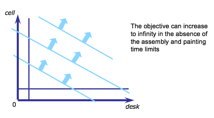
Unbounded feasible region
The telephone production problem would become unbounded if, for example, the constraints on the assembly and painting time were neglected. The feasible region would then look as in this diagram where the objective value can increase without limit, up to infinity, because there is no upper boundary to the region.
Algorithms for solving LPs
The IBM® CPLEX® Optimizers to solve LP problems in CPLEX include:
- Simplex Optimizer
- Dual-simplex Optimizer
- Barrier Optimizer
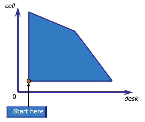
The Simplex algorithm
The Simplex algorithm, developed by George Dantzig in 1947, was the first generalized algorithm for solving LP problems. It is the basis of many optimization algorithms. The simplex method is an iterative method. It starts with an initial feasible solution, and then tests to see if it can improve the result of the objective function. It continues until the objective function cannot be further improved.
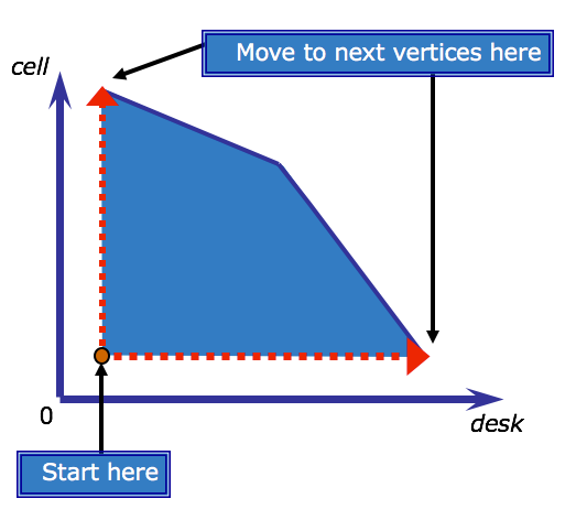
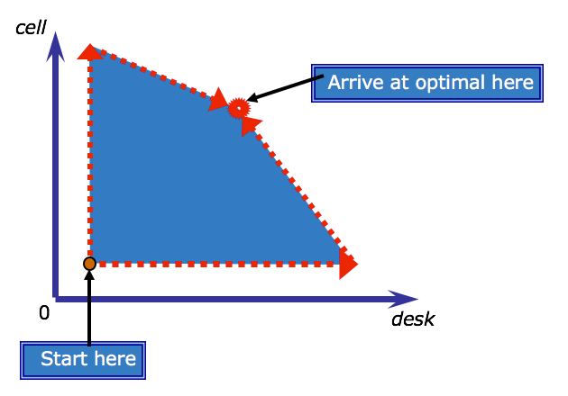
The following diagram illustrates how the simplex algorithm traverses the boundary of the feasible region for the telephone production problem. The algorithm, starts somewhere along the edge of the shaded feasible region, and advances vertex-by-vertex until arriving at the vertex that also intersects the optimal objective line. Assume it starts at the red dot indicated on the diagam.
The Revised Simplex algorithm
To improve the efficiency of the Simplex algorithm, George Dantzig and W. Orchard-Hays revised it in 1953. CPLEX uses the Revised Simplex algorithm, with a number of improvements. The CPLEX Optimizers are particularly efficient and can solve very large problems rapidly. You can tune some CPLEX Optimizer parameters to change the algorithmic behavior according to your needs.
The Dual Simplex algorithm
The dual of a LP
The concept of duality is important in Linear Programming (LP). Every LP problem has an associated LP problem known as its dual. The dual of this associated problem is the original LP problem (known as the primal problem). If the primal problem is a minimization problem, then the dual problem is a maximization problem and vice versa.
A primal-dual pair
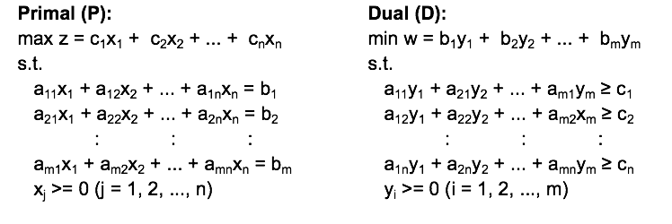
Primal (P) 
$max\ z=\sum_{i} c_{i}x_{i}$
Dual (D)
$min\ w= \sum_{j}b_{j}y_{j}$
- Each constraint in the primal has an associated dual variable, yi.
- Any feasible solution to D is an upper bound to P, and any feasible solution to P is a lower bound to D.
- In LP, the optimal objective values of D and P are equivalent, and occurs where these bounds meet.
- The dual can help solve difficult primal problems by providing a bound that in the best case equals the optimal solution to the primal problem.
Dual prices
In any solution to the dual, the values of the dual variables are known as the dual prices, also called shadow prices.
For each constraint in the primal problem, its associated dual price indicates how much the dual objective will change with a unit change in the right hand side of the constraint.
The dual price of a non-binding constraint is zero. That is, changing the right hand side of the constraint will not affect the objective value.
The dual price of a binding constraint can help you make decisions regarding the constraint.
For example, the dual price of a binding resource constraint can be used to determine whether more of the resource should be purchased or not.
The Dual Simplex algorithm
The Simplex algorithm works by finding a feasible solution and moving progressively toward optimality.
The Dual Simplex algorithm implicitly uses the dual to try and find an optimal solution to the primal as early as it can, and regardless of whether the solution is feasible or not.
It then moves from one vertex to another, gradually decreasing the infeasibility while maintaining optimality, until an optimal feasible solution to the primal problem is found.
In CPLEX, the Dual-Simplex Optimizer is the first choice for most LP problems.
Basic solutions and basic variables
You learned earlier that the Simplex algorithm travels from vertex to vertex to search for the optimal solution. A solution at a vertex is known as a basic solution. Without getting into too much detail, it's worth knowing that part of the Simplex algorithm involves setting a subset of variables to zero at each iteration. These variables are known as non-basic variables. The remaining variables are the basic variables. The concepts of basic solutions and variables are relevant in the definition of reduced costs that follows next.
Reduced Costs
The reduced cost of a variable gives an indication of the amount the objective will change with a unit increase in the variable value.
Consider the simplest form of an LP:
$ minimize\ c^{t}x\\ s.t. \\ Ax = b \\ x \ge 0 $
If $y$ represents the dual variables for a given basic solution, then the reduced costs are defined as:
$$ c - y^{t}A $$Such a basic solution is optimal if:
$$ c - y^{t}A \ge 0 $$If all reduced costs for this LP are non-negative, it follows that the objective value can only increase with a change in the variable value, and therefore the solution (when minimizing) is optimal.
DOcplex lets you acces sreduced costs of variable, after a successful solve. Let's experiment with the two decision variables of our problem:
Getting reduced cost values with DOcplex
DOcplex lets you access reduced costs of variable, after a successful solve. Let's experiment with the two decision variables of our problem:
print('* desk variable has reduced cost: {0}'.format(desk.reduced_cost))
print('* cell variable has reduced cost: {0}'.format(cell.reduced_cost))
Default optimality criteria for CPLEX optimizer
Because CPLEX Optimizer operates on finite precision computers, it uses an optimality tolerance to test the reduced costs.
The default optimality tolerance is –1e-6, with optimality criteria for the simplest form of an LP then being:
$$ c — y^{t}A> –10^{-6} $$You can adjust this optimality tolerance, for example if the algorithm takes very long to converge and has already achieved a solution sufficiently close to optimality.
Reduced Costs and multiple optimal solutions
In the earlier example you saw how one can visualize multiple optimal solutions for an LP with two variables. For larger LPs, the reduced costs can be used to determine whether multiple optimal solutions exist. Multiple optimal solutions exist when one or more non-basic variables with a zero reduced cost exist in an optimal solution (that is, variable values that can change without affecting the objective value). In order to determine whether multiple optimal solutions exist, you can examine the values of the reduced costs with DOcplex.
Slack values
For any solution, the difference between the left and right hand sides of a constraint is known as the slack value for that constraint.
For example, if a constraint states that f(x) <= 100, and in the solution f(x) = 80, then the slack value of this constraint is 20.
In the earlier example, you learned about binding and non-binding constraints. For example, f(x) <= 100 is binding if f(x) = 100, and non-binding if f(x) = 80.
The slack value for a binding constraint is always zero, that is, the constraint is met exactly.
You can determine which constraints are binding in a solution by examining the slack values with DOcplex.
This might help to better interpret the solution and help suggest which constraints may benefit from a change in bounds or a change into a soft constraint.
Accessing slack values with DOcplex
As an example, let's examine the slack values of some constraints in our problem, after we revert the change to soft constrants
# revert soft constraints
ct_assembly.rhs = 440
s3 = m.solve()

# now get slack value for assembly constraint: expected value is 40
print('* slack value for assembly time constraint is: {0}'.format(ct_assembly.slack_value))
# get slack value for painting time constraint, expected value is 0.
print('* slack value for painting time constraint is: {0}'.format(ct_painting.slack_value))
Degeneracy
It is possible that multiple non-optimal solutions with the same objective value exist.
As the simplex algorithm attempts to move in the direction of an improved objective value, it might happen that the algorithm starts cycling between non-optimal solutions with equivalent objective values. This is known as degeneracy.
Modern LP solvers, such as CPLEX Simplex Optimizer, have built-in mechanisms to help escape such cycling by using perturbation techniques involving the variable bounds.
If the default algorithm does not break the degenerate cycle, it's a good idea to try some other algorithms, for example the Dual-simplex Optimizer. Problem that are primal degenerate, are often not dual degenerate, and vice versa.
Setting a LP algorithm with DOcplex
Users can change the algorithm by editing the lpmethod parameter of the model.
We won't go into details here, it suffices to know this parameter accepts an integer from 0 to 6, where 0 denotes automatic choice of the algorithm, 1 is for primal simplex, 2 is for dual simplex, and 4 is for barrier...
For example, choosing the barrier algorithm is done by setting value 4 to this parameter. We access the parameters property of the model and from there, assign the lpmethod parameter
m.parameters.lpmethod = 4
m.solve(log_output=True)
Barrier methods
Most of the CPLEX Optimizers for MP call upon the basic simplex method or some variation of it.
Some, such as the Barrier Optimizer, use alternative methods.
In graphical terms, the Simplex Algorithm starts along the edge of the feasible region and searches for an optimal vertex.
The barrier method starts somewhere inside the feasible region – in other words, it avoids the “barrier” that is created by the constraints, and burrows through the feasible region to find the optimal solution.
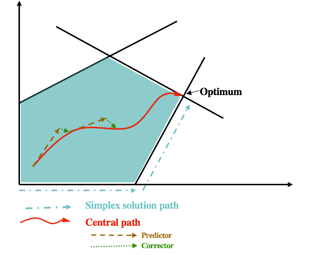
In its search, the method uses what is known as a predictor-corrector algorithm that constantly adjusts its path through the center of the feasible region (the central path).
This diagram shows how the barrier method works compared to the simplex method. As you can see, the simplex method traverses the edge of the feasible region, while the barrier method moves through the interior, with a predictor-corrector determining the path. In general, it’s a good idea to experiment with different algorithms in CPLEX when trying to improve performance.
Presolve
CPLEX Optimizer provides a presolve procedure.
Presolve evaluates the model formulation before solving it, and attempts to reduce the size of the problem that is sent to the solver engine.
A reduction in problem size typically translates to a reduction in total run time.
For example, a real problem presented to CPLEX Optimizer with approximately 160,000 constraints and 596,000 decision variables, was reduced by presolve to a problem with 27,000 constraints and 150,000 decision variables.
The presolve time was only 1.32 seconds and reduced the solution time from nearly half an hour to under 25 seconds.
An example of presolve operations
Let's consider the following Linear problem:
$ maximize:\\ [1]\ 2x_{1}+ 3x_{2} — x_{3} — x_{4}\\ subject\ to:\\ [2]\ x_{1} + x_{2} + x_{3} — 2x_{4} <= 4\\ [3]\ -x_{1} — x_{2} + x_{3} — x_{4} <= 1\\ [4]\ x_{1} + x_{4} <= 3\\ [5]\ x_{1}, x_{2}, x_{3}, x_{4} >= 0 $
- Because $x_{3}$ has a negative coefficient in the objective, the optimization will minimize $x_{3}$.
- In constraints [2] and [3] $x_{3}$ has positive coefficients, and the constraints are <=. Thus, $x_{3}$ can be reduced to 0, and becomes redundant.
- In constraint [3], all the coefficients are now negative. Because the left hand side of [3] can never be positive, any assignment of values will satisfy the constraint. The constraint is redundant and can be removed.
Summary
Having completed this notebook, you should be able to:
- Describe the characteristics of an LP in terms of the objective, decision variables and constraints
- Formulate a simple LP model on paper
- Conceptually explain the following terms in the context of LP:
- dual
- feasible region
- infeasible
- unbounded
- slacks
- reduced costs
- degeneracy
- Describe some of the algorithms used to solve LPs
- Explain what presolve does
- Write a simple LP model with DOcplex
References
- CPLEX Modeling for Python documentation
- IBM Decision Optimization
- Need help with DOcplex or to report a bug? Please go here.
- Contact us at dofeedback@wwpdl.vnet.ibm.com.