The Nurse Assignment Problem¶

This tutorial includes everything you need to set up IBM Decision Optimization CPLEX Modeling for Python (DOcplex), build a Mathematical Programming model, and get its solution by solving the model on the cloud with IBM ILOG CPLEX Optimizer.

When you finish this tutorial, you’ll have a foundational knowledge of Prescriptive Analytics.

This notebook is part of Prescriptive Analytics for Python

It requires either an installation of CPLEX Optimizers or it can be run on IBM Watson Studio Cloud (Sign up for a free IBM Cloud account and you can start using Watson Studio Cloud right away).

Table of contents:

Describe the business problem
How decision optimization can help
Use decision optimization
Summary

Describe the business problem¶

This notebook describes how to use CPLEX Modeling for Python together with pandas to manage the assignment of nurses to shifts in a hospital.

Nurses must be assigned to hospital shifts in accordance with various skill and staffing constraints.

The goal of the model is to find an efficient balance between the different objectives:

minimize the overall cost of the plan and
assign shifts as fairly as possible.

How decision optimization can help¶

Prescriptive analytics (decision optimization) technology recommends actions that are based on desired outcomes. It takes into account specific scenarios, resources, and knowledge of past and current events. With this insight, your organization can make better decisions and have greater control of business outcomes.
Prescriptive analytics is the next step on the path to insight-based actions. It creates value through synergy with predictive analytics, which analyzes data to predict future outcomes.
Prescriptive analytics takes that insight to the next level by suggesting the optimal way to handle that future situation. Organizations that can act fast in dynamic conditions and make superior decisions in uncertain environments gain a strong competitive advantage.

With prescriptive analytics, you can:

Automate the complex decisions and trade-offs to better manage your limited resources.
Take advantage of a future opportunity or mitigate a future risk.
Proactively update recommendations based on changing events.
Meet operational goals, increase customer loyalty, prevent threats and fraud, and optimize business processes.

Checking minimum requirements¶

This notebook uses some features of pandas that are available in version 0.17.1 or above.

Use decision optimization¶

Step 1: Import the library¶

Run the following code to import the Decision Optimization CPLEX Modeling library. The DOcplex library contains the two modeling packages, Mathematical Programming (docplex.mp) and Constraint Programming (docplex.cp).

Step 2: Model the data¶

The input data consists of several tables:

The Departments table lists all departments in the scope of the assignment.
The Skills table list all skills.
The Shifts table lists all shifts to be staffed. A shift contains a department, a day in the week, plus the start and end times.
The Nurses table lists all nurses, identified by their names.
The NurseSkills table gives the skills of each nurse.
The SkillRequirements table lists the minimum number of persons required for a given department and skill.
The NurseVacations table lists days off for each nurse.
The NurseAssociations table lists pairs of nurses who wish to work together.
The NurseIncompatibilities table lists pairs of nurses who do not want to work together.

Loading data from Excel with pandas¶

We load the data from an Excel file using pandas. Each sheet is read into a separate pandas DataFrame.

#nurses = 32
#shifts = 41
#vacations = 59

In addition, we introduce some extra global data:

The maximum work time for each nurse.
The maximum and minimum number of shifts worked by a nurse in a week.

Shifts are stored in a separate DataFrame.

	department	day	start_time	end_time	min_req	max_req
shiftId
0	Emergency	Monday	2	8	3	5
1	Emergency	Monday	8	12	4	7
2	Emergency	Monday	12	18	2	5
3	Emergency	Monday	18	2	3	7
4	Consultation	Monday	8	12	10	13
5	Consultation	Monday	12	18	8	12
6	Cardiac Care	Monday	8	12	10	13
7	Cardiac Care	Monday	12	18	8	12
8	Emergency	Tuesday	8	12	4	7
9	Emergency	Tuesday	12	18	2	5
10	Emergency	Tuesday	18	2	3	7
11	Consultation	Tuesday	8	12	10	13
12	Consultation	Tuesday	12	18	8	12
13	Cardiac Care	Tuesday	8	12	4	7
14	Cardiac Care	Tuesday	12	18	2	5
15	Cardiac Care	Tuesday	18	2	3	7
16	Emergency	Wednesday	2	8	3	5
17	Emergency	Wednesday	8	12	4	7
18	Emergency	Wednesday	12	18	2	5
19	Emergency	Wednesday	18	2	3	7
20	Consultation	Wednesday	8	12	10	13
21	Consultation	Wednesday	12	18	8	12
22	Emergency	Thursday	2	8	3	5
23	Emergency	Thursday	8	12	4	7
24	Emergency	Thursday	12	18	2	5
25	Emergency	Thursday	18	2	3	7
26	Consultation	Thursday	8	12	10	13
27	Consultation	Thursday	12	18	8	12
28	Emergency	Friday	2	8	3	5
29	Emergency	Friday	8	12	4	7
30	Emergency	Friday	12	18	2	5
31	Emergency	Friday	18	2	3	7
32	Consultation	Friday	8	12	10	13
33	Consultation	Friday	12	18	8	12
34	Emergency	Saturday	2	12	5	7
35	Emergency	Saturday	12	20	7	9
36	Emergency	Saturday	20	2	12	12
37	Emergency	Sunday	2	12	5	7
38	Emergency	Sunday	12	20	7	9
39	Emergency	Sunday	20	2	8	12
40	Geriatrics	Sunday	8	10	2	5

Step 3: Prepare the data¶

We need to precompute additional data for shifts. For each shift, we need the start time and end time expressed in hours, counting from the beginning of the week: Monday 8am is converted to 8, Tuesday 8am is converted to 24+8 = 32, and so on.

Sub-step #1¶

We start by adding an extra column dow (day of week) which converts the string “day” into an integer in 0..6 (Monday is 0, Sunday is 6).

	department	day	start_time	end_time	min_req	max_req	dow
shiftId
0	Emergency	Monday	2	8	3	5	0
1	Emergency	Monday	8	12	4	7	0
2	Emergency	Monday	12	18	2	5	0
3	Emergency	Monday	18	2	3	7	0
4	Consultation	Monday	8	12	10	13	0
5	Consultation	Monday	12	18	8	12	0
6	Cardiac Care	Monday	8	12	10	13	0
7	Cardiac Care	Monday	12	18	8	12	0
8	Emergency	Tuesday	8	12	4	7	1
9	Emergency	Tuesday	12	18	2	5	1
10	Emergency	Tuesday	18	2	3	7	1
11	Consultation	Tuesday	8	12	10	13	1
12	Consultation	Tuesday	12	18	8	12	1
13	Cardiac Care	Tuesday	8	12	4	7	1
14	Cardiac Care	Tuesday	12	18	2	5	1
15	Cardiac Care	Tuesday	18	2	3	7	1
16	Emergency	Wednesday	2	8	3	5	2
17	Emergency	Wednesday	8	12	4	7	2
18	Emergency	Wednesday	12	18	2	5	2
19	Emergency	Wednesday	18	2	3	7	2
20	Consultation	Wednesday	8	12	10	13	2
21	Consultation	Wednesday	12	18	8	12	2
22	Emergency	Thursday	2	8	3	5	3
23	Emergency	Thursday	8	12	4	7	3
24	Emergency	Thursday	12	18	2	5	3
25	Emergency	Thursday	18	2	3	7	3
26	Consultation	Thursday	8	12	10	13	3
27	Consultation	Thursday	12	18	8	12	3
28	Emergency	Friday	2	8	3	5	4
29	Emergency	Friday	8	12	4	7	4
30	Emergency	Friday	12	18	2	5	4
31	Emergency	Friday	18	2	3	7	4
32	Consultation	Friday	8	12	10	13	4
33	Consultation	Friday	12	18	8	12	4
34	Emergency	Saturday	2	12	5	7	5
35	Emergency	Saturday	12	20	7	9	5
36	Emergency	Saturday	20	2	12	12	5
37	Emergency	Sunday	2	12	5	7	6
38	Emergency	Sunday	12	20	7	9	6
39	Emergency	Sunday	20	2	8	12	6
40	Geriatrics	Sunday	8	10	2	5	6

Sub-step #2 : Compute the absolute start time of each shift.¶

Computing the start time in the week is easy: just add 24*dow to column start_time. The result is stored in a new column wstart.

Sub-Step #3 : Compute the absolute end time of each shift.¶

Computing the absolute end time is a little more complicated as certain shifts span across midnight. For example, Shift #3 starts on Monday at 18:00 and ends Tuesday at 2:00 AM. The absolute end time of Shift #3 is 26, not 2. The general rule for computing absolute end time is:

abs_end_time = end_time + 24 * dow + (start_time>= end_time ? 24 : 0)

Again, we use pandas to add a new calculated column wend. This is done by using the pandas apply method with an anonymous lambda function over rows. The raw=True parameter prevents the creation of a pandas Series for each row, which improves the performance significantly on large data sets.

Sub-step #4 : Compute the duration of each shift.¶

Computing the duration of each shift is now a straightforward difference of columns. The result is stored in column duration.

Sub-step #5 : Compute the minimum demand for each shift.¶

Minimum demand is the product of duration (in hours) by the minimum required number of nurses. Thus, in number of nurse-hours, this demand is stored in another new column min_demand.

Finally, we display the updated shifts DataFrame with all calculated columns.

	department	day	start_time	end_time	min_req	max_req	dow	wstart	wend	duration	min_demand
shiftId
0	Emergency	Monday	2	8	3	5	0	2	8	6	18
1	Emergency	Monday	8	12	4	7	0	8	12	4	16
2	Emergency	Monday	12	18	2	5	0	12	18	6	12
3	Emergency	Monday	18	2	3	7	0	18	26	8	24
4	Consultation	Monday	8	12	10	13	0	8	12	4	40
5	Consultation	Monday	12	18	8	12	0	12	18	6	48
6	Cardiac Care	Monday	8	12	10	13	0	8	12	4	40
7	Cardiac Care	Monday	12	18	8	12	0	12	18	6	48
8	Emergency	Tuesday	8	12	4	7	1	32	36	4	16
9	Emergency	Tuesday	12	18	2	5	1	36	42	6	12
10	Emergency	Tuesday	18	2	3	7	1	42	50	8	24
11	Consultation	Tuesday	8	12	10	13	1	32	36	4	40
12	Consultation	Tuesday	12	18	8	12	1	36	42	6	48
13	Cardiac Care	Tuesday	8	12	4	7	1	32	36	4	16
14	Cardiac Care	Tuesday	12	18	2	5	1	36	42	6	12
15	Cardiac Care	Tuesday	18	2	3	7	1	42	50	8	24
16	Emergency	Wednesday	2	8	3	5	2	50	56	6	18
17	Emergency	Wednesday	8	12	4	7	2	56	60	4	16
18	Emergency	Wednesday	12	18	2	5	2	60	66	6	12
19	Emergency	Wednesday	18	2	3	7	2	66	74	8	24
20	Consultation	Wednesday	8	12	10	13	2	56	60	4	40
21	Consultation	Wednesday	12	18	8	12	2	60	66	6	48
22	Emergency	Thursday	2	8	3	5	3	74	80	6	18
23	Emergency	Thursday	8	12	4	7	3	80	84	4	16
24	Emergency	Thursday	12	18	2	5	3	84	90	6	12
25	Emergency	Thursday	18	2	3	7	3	90	98	8	24
26	Consultation	Thursday	8	12	10	13	3	80	84	4	40
27	Consultation	Thursday	12	18	8	12	3	84	90	6	48
28	Emergency	Friday	2	8	3	5	4	98	104	6	18
29	Emergency	Friday	8	12	4	7	4	104	108	4	16
30	Emergency	Friday	12	18	2	5	4	108	114	6	12
31	Emergency	Friday	18	2	3	7	4	114	122	8	24
32	Consultation	Friday	8	12	10	13	4	104	108	4	40
33	Consultation	Friday	12	18	8	12	4	108	114	6	48
34	Emergency	Saturday	2	12	5	7	5	122	132	10	50
35	Emergency	Saturday	12	20	7	9	5	132	140	8	56
36	Emergency	Saturday	20	2	12	12	5	140	146	6	72
37	Emergency	Sunday	2	12	5	7	6	146	156	10	50
38	Emergency	Sunday	12	20	7	9	6	156	164	8	56
39	Emergency	Sunday	20	2	8	12	6	164	170	6	48
40	Geriatrics	Sunday	8	10	2	5	6	152	154	2	4

Step 4: Set up the prescriptive model¶

* system is: Windows 64bit
* Python version 3.7.3, located at: c:\local\python373\python.exe
* docplex is present, version is (2, 11, 0)
* pandas is present, version is 0.25.1

Create the DOcplex model¶

The model contains all the business constraints and defines the objective.

We now use CPLEX Modeling for Python to build a Mixed Integer Programming (MIP) model for this problem.

Define the decision variables¶

For each (nurse, shift) pair, we create one binary variable that is equal to 1 when the nurse is assigned to the shift.

We use the binary_var_matrix method of class Model, as each binary variable is indexed by two objects: one nurse and one shift.

Express the business constraints¶

Overlapping shifts¶

Some shifts overlap in time, and thus cannot be assigned to the same nurse. To check whether two shifts overlap in time, we start by ordering all shifts with respect to their wstart and duration properties. Then, for each shift, we iterate over the subsequent shifts in this ordered list to easily compute the subset of overlapping shifts.

We use pandas operations to implement this algorithm. But first, we organize all decision variables in a DataFrame.

For convenience, we also organize the decision variables in a pivot table with nurses as row index and shifts as columns. The pandas unstack operation does this.

	assigned
all_shifts	0	1	2	3	4	5	6	7	8	9	...	31	32	33	34	35	36	37	38	39	40
all_nurses
Anne	assign_Anne_0	assign_Anne_1	assign_Anne_2	assign_Anne_3	assign_Anne_4	assign_Anne_5	assign_Anne_6	assign_Anne_7	assign_Anne_8	assign_Anne_9	...	assign_Anne_31	assign_Anne_32	assign_Anne_33	assign_Anne_34	assign_Anne_35	assign_Anne_36	assign_Anne_37	assign_Anne_38	assign_Anne_39	assign_Anne_40
Bethanie	assign_Bethanie_0	assign_Bethanie_1	assign_Bethanie_2	assign_Bethanie_3	assign_Bethanie_4	assign_Bethanie_5	assign_Bethanie_6	assign_Bethanie_7	assign_Bethanie_8	assign_Bethanie_9	...	assign_Bethanie_31	assign_Bethanie_32	assign_Bethanie_33	assign_Bethanie_34	assign_Bethanie_35	assign_Bethanie_36	assign_Bethanie_37	assign_Bethanie_38	assign_Bethanie_39	assign_Bethanie_40
Betsy	assign_Betsy_0	assign_Betsy_1	assign_Betsy_2	assign_Betsy_3	assign_Betsy_4	assign_Betsy_5	assign_Betsy_6	assign_Betsy_7	assign_Betsy_8	assign_Betsy_9	...	assign_Betsy_31	assign_Betsy_32	assign_Betsy_33	assign_Betsy_34	assign_Betsy_35	assign_Betsy_36	assign_Betsy_37	assign_Betsy_38	assign_Betsy_39	assign_Betsy_40
Cathy	assign_Cathy_0	assign_Cathy_1	assign_Cathy_2	assign_Cathy_3	assign_Cathy_4	assign_Cathy_5	assign_Cathy_6	assign_Cathy_7	assign_Cathy_8	assign_Cathy_9	...	assign_Cathy_31	assign_Cathy_32	assign_Cathy_33	assign_Cathy_34	assign_Cathy_35	assign_Cathy_36	assign_Cathy_37	assign_Cathy_38	assign_Cathy_39	assign_Cathy_40
Cecilia	assign_Cecilia_0	assign_Cecilia_1	assign_Cecilia_2	assign_Cecilia_3	assign_Cecilia_4	assign_Cecilia_5	assign_Cecilia_6	assign_Cecilia_7	assign_Cecilia_8	assign_Cecilia_9	...	assign_Cecilia_31	assign_Cecilia_32	assign_Cecilia_33	assign_Cecilia_34	assign_Cecilia_35	assign_Cecilia_36	assign_Cecilia_37	assign_Cecilia_38	assign_Cecilia_39	assign_Cecilia_40

5 rows � 41 columns

We create a DataFrame representing a list of shifts sorted by “wstart” and “duration”. This sorted list will be used to easily detect overlapping shifts.

Note that indices are reset after sorting so that the DataFrame can be indexed with respect to the index in the sorted list and not the original unsorted list. This is the purpose of the reset_index() operation which also adds a new column named “shiftId” with the original index.

	shiftId	wstart	wend
0	0	2	8
1	1	8	12
2	4	8	12
3	6	8	12
4	2	12	18

Next, we state that for any pair of shifts that overlap in time, a nurse can be assigned to only one of the two.

#incompatible shift constraints: 640

Vacations¶

When the nurse is on vacation, he cannot be assigned to any shift starting that day.

We use the pandas merge operation to create a join between the “df_vacations”, “df_shifts”, and “df_assigned” DataFrames. Each row of the resulting DataFrame contains the assignment decision variable corresponding to the matching (nurse, shift) pair.

	nurse	day	dow	shiftId	all_nurses	all_shifts	assigned
0	Anne	Friday	4	28	Anne	28	assign_Anne_28
1	Anne	Friday	4	29	Anne	29	assign_Anne_29
2	Anne	Friday	4	30	Anne	30	assign_Anne_30
3	Anne	Friday	4	31	Anne	31	assign_Anne_31
4	Anne	Friday	4	32	Anne	32	assign_Anne_32

# vacation forbids: 342 assignments

Associations¶

Some pairs of nurses get along particularly well, so we wish to assign them together as a team. In other words, for every such couple and for each shift, both assignment variables should always be equal. Either both nurses work the shift, or both do not.

In the same way we modeled vacations, we use the pandas merge operation to create a DataFrame for which each row contains the pair of nurse-shift assignment decision variables matching each association.

	nurse1	nurse2	all_nurses_1	all_shifts	assigned_1	all_nurses_2	assigned_2
0	Isabelle	Dee	Isabelle	0	assign_Isabelle_0	Dee	assign_Dee_0
1	Isabelle	Dee	Isabelle	1	assign_Isabelle_1	Dee	assign_Dee_1
2	Isabelle	Dee	Isabelle	2	assign_Isabelle_2	Dee	assign_Dee_2
3	Isabelle	Dee	Isabelle	3	assign_Isabelle_3	Dee	assign_Dee_3
4	Isabelle	Dee	Isabelle	4	assign_Isabelle_4	Dee	assign_Dee_4

The associations constraint can now easily be formulated by iterating on the rows of the “df_preferred_assign” DataFrame.

Incompatibilities¶

Similarly, certain pairs of nurses do not get along well, and we want to avoid having them together on a shift. In other terms, for each shift, both nurses of an incompatible pair cannot be assigned together to the sift. Again, we state a logical OR between the two assignments: at most one nurse from the pair can work the shift.

We first create a DataFrame whose rows contain pairs of invalid assignment decision variables, using the same pandas merge operations as in the previous step.

	nurse1	nurse2	all_nurses_1	all_shifts	assigned_1	all_nurses_2	assigned_2
0	Patricia	Patrick	Patricia	0	assign_Patricia_0	Patrick	assign_Patrick_0
1	Patricia	Patrick	Patricia	1	assign_Patricia_1	Patrick	assign_Patrick_1
2	Patricia	Patrick	Patricia	2	assign_Patricia_2	Patrick	assign_Patrick_2
3	Patricia	Patrick	Patricia	3	assign_Patricia_3	Patrick	assign_Patrick_3
4	Patricia	Patrick	Patricia	4	assign_Patricia_4	Patrick	assign_Patrick_4

The incompatibilities constraint can now easily be formulated, by iterating on the rows of the “df_incompatible_assign” DataFrame.

Constraints on work time¶

Regulations force constraints on the total work time over a week; and we compute this total work time in a new variable. We store the variable in an extra column in the nurse DataFrame.

The variable is declared as continuous though it contains only integer values. This is done to avoid adding unnecessary integer variables for the branch and bound algorithm. These variables are not true decision variables; they are used to express work constraints.

From a pandas perspective, we apply a function over the rows of the nurse DataFrame to create this variable and store it into a new column of the DataFrame.

	seniority	qualification	pay_rate	worktime
name
Anne	11	1	25	worktime_Anne
Bethanie	4	5	28	worktime_Bethanie
Betsy	2	2	17	worktime_Betsy
Cathy	2	2	17	worktime_Cathy
Cecilia	9	5	38	worktime_Cecilia
Chris	11	4	38	worktime_Chris
Cindy	5	2	21	worktime_Cindy
David	1	2	15	worktime_David
Debbie	7	2	24	worktime_Debbie
Dee	3	3	21	worktime_Dee
Gloria	8	2	25	worktime_Gloria
Isabelle	3	1	16	worktime_Isabelle
Jane	3	4	23	worktime_Jane
Janelle	4	3	22	worktime_Janelle
Janice	2	2	17	worktime_Janice
Jemma	2	4	22	worktime_Jemma
Joan	5	3	24	worktime_Joan
Joyce	8	3	29	worktime_Joyce
Jude	4	3	22	worktime_Jude
Julie	6	2	22	worktime_Julie
Juliet	7	4	31	worktime_Juliet
Kate	5	3	24	worktime_Kate
Nancy	8	4	32	worktime_Nancy
Nathalie	9	5	38	worktime_Nathalie
Nicole	0	2	14	worktime_Nicole
Patricia	1	1	13	worktime_Patricia
Patrick	6	1	19	worktime_Patrick
Roberta	3	5	26	worktime_Roberta
Suzanne	5	1	18	worktime_Suzanne
Vickie	7	1	20	worktime_Vickie
Wendie	5	2	21	worktime_Wendie
Zoe	8	3	29	worktime_Zoe

Define total work time

Work time variables must be constrained to be equal to the sum of hours actually worked.

We use the pandas groupby operation to collect all assignment decision variables for each nurse in a separate series. Then, we iterate over nurses to post a constraint calculating the actual worktime for each nurse as the dot product of the series of nurse-shift assignments with the series of shift durations.

Model: nurses
 - number of variables: 1344
   - binary=1312, integer=0, continuous=32
 - number of constraints: 1547
   - linear=1547
 - parameters: defaults
 - problem type is: MILP

Maximum work time

For each nurse, we add a constraint to enforce the maximum work time for a week. Again we use the apply method, this time with an anonymous lambda function.

name
Anne            worktime_Anne <= 40
Bethanie    worktime_Bethanie <= 40
Betsy          worktime_Betsy <= 40
Cathy          worktime_Cathy <= 40
Cecilia      worktime_Cecilia <= 40
Chris          worktime_Chris <= 40
Cindy          worktime_Cindy <= 40
David          worktime_David <= 40
Debbie        worktime_Debbie <= 40
Dee              worktime_Dee <= 40
Gloria        worktime_Gloria <= 40
Isabelle    worktime_Isabelle <= 40
Jane            worktime_Jane <= 40
Janelle      worktime_Janelle <= 40
Janice        worktime_Janice <= 40
Jemma          worktime_Jemma <= 40
Joan            worktime_Joan <= 40
Joyce          worktime_Joyce <= 40
Jude            worktime_Jude <= 40
Julie          worktime_Julie <= 40
Juliet        worktime_Juliet <= 40
Kate            worktime_Kate <= 40
Nancy          worktime_Nancy <= 40
Nathalie    worktime_Nathalie <= 40
Nicole        worktime_Nicole <= 40
Patricia    worktime_Patricia <= 40
Patrick      worktime_Patrick <= 40
Roberta      worktime_Roberta <= 40
Suzanne      worktime_Suzanne <= 40
Vickie        worktime_Vickie <= 40
Wendie        worktime_Wendie <= 40
Zoe              worktime_Zoe <= 40
Name: worktime, dtype: object

Minimum requirement for shifts¶

Each shift requires a minimum number of nurses. For each shift, the sum over all nurses of assignments to this shift must be greater than the minimum requirement.

The pandas groupby operation is invoked to collect all assignment decision variables for each shift in a separate series. Then, we iterate over shifts to post the constraint enforcing the minimum number of nurse assignments for each shift.

Express the objective¶

The objective mixes different (and contradictory) KPIs.

The first KPI is the total salary cost, computed as the sum of work times over all nurses, weighted by pay rate.

We compute this KPI as an expression from the variables we previously defined by using the panda summation over the DOcplex objects.

DecisionKPI(name=Total salary cost,expr=25worktime_Anne+28worktime_Bethanie+17worktime_Betsy+17worktime_..)

Minimizing salary cost¶

In a preliminary version of the model, we minimize the total salary cost. This is accomplished using the Model.minimize() method.

Model: nurses
 - number of variables: 1344
   - binary=1312, integer=0, continuous=32
 - number of constraints: 1588
   - linear=1588
 - parameters: defaults
 - problem type is: MILP

Solve with Decision Optimization¶

Now we have everything we need to solve the model, using Model.solve(). The following cell solves using your local CPLEX (if any, and provided you have added it to your PYTHONPATH variable).

CPXPARAM_Read_DataCheck                          1
CPXPARAM_MIP_Tolerances_MIPGap                   1.0000000000000001e-05
Tried aggregator 2 times.
MIP Presolve eliminated 997 rows and 379 columns.
MIP Presolve modified 90 coefficients.
Aggregator did 41 substitutions.
Reduced MIP has 550 rows, 922 columns, and 2862 nonzeros.
Reduced MIP has 892 binaries, 0 generals, 0 SOSs, and 0 indicators.
Presolve time = 0.00 sec. (3.68 ticks)
Probing time = 0.00 sec. (0.50 ticks)
Tried aggregator 1 time.
Reduced MIP has 550 rows, 922 columns, and 2862 nonzeros.
Reduced MIP has 892 binaries, 30 generals, 0 SOSs, and 0 indicators.
Presolve time = 0.00 sec. (2.03 ticks)
Probing time = 0.00 sec. (0.50 ticks)
Clique table members: 479.
MIP emphasis: balance optimality and feasibility.
MIP search method: dynamic search.
Parallel mode: deterministic, using up to 12 threads.
Root relaxation solution time = 0.00 sec. (4.56 ticks)

        Nodes                                         Cuts/
   Node  Left     Objective  IInf  Best Integer    Best Bound    ItCnt     Gap

      0     0    28824.0000    48                  28824.0000      473
      0     0    28824.0000    62                    Cuts: 98      649
      0     0    28824.0000    35                    Cuts: 44      716
      0     0    28824.0000    41                    Cuts: 55      795
*     0+    0                        29100.0000    28824.0000             0.95%
*     0+    0                        29068.0000    28824.0000             0.84%
      0     2    28824.0000    10    29068.0000    28824.0000      795    0.84%
Elapsed time = 0.24 sec. (139.30 ticks, tree = 0.02 MB, solutions = 2)
*    10+    4                        29014.0000    28824.0000             0.65%
*    11+    2                        29010.0000    28824.0000             0.64%
*    15+    2                        28982.0000    28824.0000             0.55%
*    26+    1                        28944.0000    28824.0000             0.41%
*    47+   10                        28936.0000    28824.0000             0.39%
*  1611+ 1392                        28888.0000    28824.0000             0.22%
*  4006+ 3397                        28842.0000    28824.0000             0.06%
*  4152+ 3293                        28824.0000    28824.0000             0.00%
   4253  3414    28824.0000     6    28824.0000    28824.0000    73849    0.00%

GUB cover cuts applied:  12
Cover cuts applied:  76
Flow cuts applied:  5
Mixed integer rounding cuts applied:  11
Zero-half cuts applied:  13
Lift and project cuts applied:  5

Root node processing (before b&c):
  Real time             =    0.24 sec. (139.27 ticks)
Parallel b&c, 12 threads:
  Real time             =    0.47 sec. (270.80 ticks)
  Sync time (average)   =    0.08 sec.
  Wait time (average)   =    0.00 sec.
                          ------------
Total (root+branch&cut) =    0.70 sec. (410.07 ticks)
* model nurses solved with objective = 28824.000
*  KPI: Total salary cost = 28824.000

Step 5: Investigate the solution and then run an example analysis¶

We take advantage of pandas to analyze the results. First we store the solution values of the assignment variables into a new pandas Series.

Calling solution_value on a DOcplex variable returns its value in the solution (provided the model has been successfully solved).

all_shifts	0	1	2	3	4	5	6	7	8	9	...	31	32	33	34	35	36	37	38	39	40
all_nurses
Anne	0.0	1.0	0.0	0.0	0.0	1.0	0.0	0.0	0.0	0.0	...	0.0	0.0	0.0	0.0	0.0	0.0	0.0	0.0	0.0	0.0
Bethanie	0.0	1.0	0.0	0.0	0.0	0.0	0.0	1.0	0.0	0.0	...	0.0	0.0	1.0	1.0	0.0	0.0	0.0	0.0	0.0	0.0
Betsy	0.0	0.0	0.0	0.0	0.0	0.0	0.0	0.0	0.0	0.0	...	1.0	1.0	0.0	0.0	0.0	0.0	0.0	0.0	0.0	0.0
Cathy	0.0	0.0	0.0	0.0	0.0	0.0	1.0	1.0	0.0	0.0	...	0.0	1.0	1.0	0.0	0.0	1.0	1.0	0.0	0.0	0.0
Cecilia	0.0	0.0	0.0	1.0	0.0	1.0	1.0	0.0	0.0	0.0	...	0.0	0.0	0.0	0.0	0.0	0.0	0.0	0.0	0.0	0.0

5 rows � 41 columns

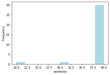
Analyzing how worktime is distributed¶

Let’s analyze how worktime is distributed among nurses.

First, we compute the global average work time as the total minimum requirement in hours, divided by number of nurses.

* theoretical average work time is 39 h

Let’s analyze the series of deviations to the average, stored in a pandas Series.

* the sum of absolute deviations from mean is 58.0

To see how work time is distributed among nurses, print a histogram of work time values. Note that, as all time data are integers, work times in the solution can take only integer values.

Text(0.5, 0, 'worktime')

How shifts are distributed¶

Let’s now analyze the solution from the number of shifts perspective. How many shifts does each nurse work? Are these shifts fairly distributed amongst nurses?

We compute a new column in our result DataFrame for the number of shifts worked, by summing rows (the “axis=1” argument in the sum() call indicates to pandas that each sum is performed by row instead of column):

Text(0, 0.5, '#shifts worked')

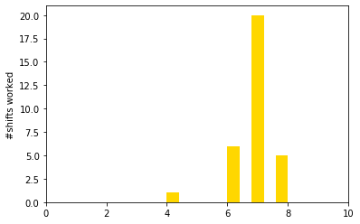
We see that one nurse works significantly fewer shifts than others do. What is the average number of shifts worked by a nurse? This is equal to the total demand divided by the number of nurses.

Of course, this yields a fractional number of shifts that is not practical, but nonetheless will help us quantify the fairness in shift distribution.

-- expected avg #shifts worked is 6.875
-- total absolute deviation to mean #shifts is 16.25

Introducing a fairness goal¶

As the above diagram suggests, the distribution of shifts could be improved. We implement this by adding one extra objective, fairness, which balances the shifts assigned over nurses.

Note that we can edit the model, that is add (or remove) constraints, even after it has been solved.

Step #1 : Introduce three new variables per nurse to model the¶

number of shifts worked and positive and negative deviations to the average.

Step #2 : Post the constraint that links these variables together.¶

Step #3 : Define KPIs to measure the result after solve.¶

DecisionKPI(name=Total under-worked,expr=underw_Anne+underw_Bethanie+underw_Betsy+underw_Cathy+underw_Cec..)

Finally, let’s modify the objective by adding the sum of over_worked and under_worked to the previous objective.

Note: The definitions of over_worked and under_worked as described above are not sufficient to give them an unambiguous value. However, as all these variables are minimized, CPLEX ensures that these variables take the minimum possible values in the solution.

Our modified model is ready to solve.

The log_output=True parameter tells CPLEX to print the log on the standard output.

CPXPARAM_Read_DataCheck                          1
CPXPARAM_MIP_Tolerances_MIPGap                   1.0000000000000001e-05
1 of 31 MIP starts provided solutions.
MIP start 'm1' defined initial solution with objective 28840.2500.
Tried aggregator 2 times.
MIP Presolve eliminated 997 rows and 379 columns.
MIP Presolve modified 90 coefficients.
Aggregator did 73 substitutions.
Reduced MIP has 582 rows, 986 columns, and 3859 nonzeros.
Reduced MIP has 892 binaries, 0 generals, 0 SOSs, and 0 indicators.
Presolve time = 0.02 sec. (4.35 ticks)
Probing time = 0.00 sec. (0.59 ticks)
Tried aggregator 1 time.
MIP Presolve eliminated 2 rows and 4 columns.
Reduced MIP has 580 rows, 982 columns, and 3814 nonzeros.
Reduced MIP has 892 binaries, 30 generals, 0 SOSs, and 0 indicators.
Presolve time = 0.00 sec. (2.41 ticks)
Probing time = 0.00 sec. (0.58 ticks)
Clique table members: 479.
MIP emphasis: balance optimality and feasibility.
MIP search method: dynamic search.
Parallel mode: deterministic, using up to 12 threads.
Root relaxation solution time = 0.01 sec. (11.48 ticks)

        Nodes                                         Cuts/
   Node  Left     Objective  IInf  Best Integer    Best Bound    ItCnt     Gap

*     0+    0                        28840.2500        0.0000           100.00%
      0     0    28827.9167    76    28840.2500    28827.9167      885    0.04%
      0     0    28829.2500    51    28840.2500      Cuts: 89     1053    0.04%
      0     0    28829.9063    59    28840.2500     Cuts: 107     1359    0.04%
      0     0    28831.0000    33    28840.2500      Cuts: 55     1530    0.03%
      0     0    28831.0000    45    28840.2500      Cuts: 36     1649    0.03%
      0     0    28831.0000    35    28840.2500       Cuts: 8     1715    0.03%
      0     0    28831.0000    34    28840.2500      Cuts: 29     1783    0.03%
*     0+    0                        28831.2500    28831.0000             0.00%

GUB cover cuts applied:  19
Cover cuts applied:  4
Flow cuts applied:  21
Mixed integer rounding cuts applied:  69
Zero-half cuts applied:  14
Gomory fractional cuts applied:  4

Root node processing (before b&c):
  Real time             =    0.36 sec. (211.92 ticks)
Parallel b&c, 12 threads:
  Real time             =    0.00 sec. (0.00 ticks)
  Sync time (average)   =    0.00 sec.
  Wait time (average)   =    0.00 sec.
                          ------------
Total (root+branch&cut) =    0.36 sec. (211.92 ticks)
* model nurses solved with objective = 28831.250
*  KPI: Total salary cost  = 28824.000
*  KPI: Total over-worked  = 3.625
*  KPI: Total under-worked = 3.625

Analyzing new results¶

Let’s recompute the new total deviation from average on this new solution.

-- total absolute deviation to mean #shifts is now 7.25 down from 16.25

all_shifts	0	1	2	3	4	5	6	7	8	9	...	32	33	34	35	36	37	38	39	40	worked
all_nurses
Anne	0.0	1.0	0.0	1.0	0.0	0.0	0.0	0.0	0.0	1.0	...	0.0	0.0	0.0	0.0	0.0	0.0	0.0	0.0	0.0	7.0
Bethanie	0.0	0.0	0.0	0.0	1.0	0.0	0.0	1.0	0.0	0.0	...	0.0	1.0	1.0	0.0	0.0	0.0	0.0	0.0	0.0	7.0
Betsy	0.0	0.0	0.0	0.0	0.0	0.0	0.0	0.0	1.0	0.0	...	1.0	1.0	1.0	0.0	0.0	0.0	0.0	0.0	0.0	7.0
Cathy	0.0	0.0	0.0	0.0	0.0	0.0	1.0	0.0	0.0	0.0	...	0.0	1.0	0.0	0.0	1.0	1.0	0.0	1.0	0.0	7.0
Cecilia	0.0	0.0	0.0	0.0	0.0	1.0	1.0	0.0	0.0	0.0	...	0.0	0.0	0.0	0.0	1.0	0.0	0.0	0.0	0.0	7.0

5 rows � 42 columns

Let’s print the new histogram of shifts worked.

<matplotlib.axes._subplots.AxesSubplot at 0x279df51e710>

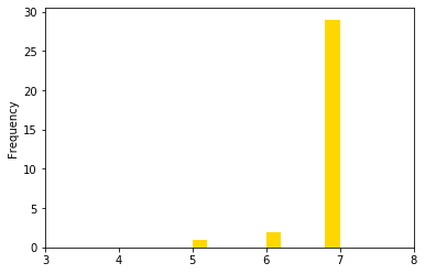
The breakdown of shifts over nurses is much closer to the average than it was in the previous version.

But what would be the minimal fairness level?¶

But what is the absolute minimum for the deviation to the ideal average number of shifts? CPLEX can tell us: simply minimize only the the total deviation from average, ignoring the salary cost. Of course this is unrealistic, but it will help us quantify how far our fairness result is to the absolute optimal fairness.

We modify the objective and solve for the third time.

* model nurses solved with objective = 4.000
*  KPI: Total salary cost  = 29606.000
*  KPI: Total over-worked  = 4.000
*  KPI: Total under-worked = 0.000

In the fairness-optimal solution, we have zero under-average shifts and 4 over-average. Salary cost is now higher than the previous value of 28884 but this was expected as salary cost was not part of the objective.

To summarize, the absolute minimum for this measure of fairness is 4, and we have found a balance with fairness=7.

Finally, we display the histogram for this optimal-fairness solution.

<matplotlib.axes._subplots.AxesSubplot at 0x279e05915f8>

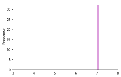
In the above figure, all nurses but one are assigned the average of 7 shifts, which is what we expected.

Summary¶

You learned how to set up and use IBM Decision Optimization CPLEX Modeling for Python to formulate a Mathematical Programming model and solve it with IBM Decision Optimization on Cloud.

References¶

CPLEX Modeling for Python documentation
Decision Optimization on Cloud
Need help with DOcplex or to report a bug? Please go here.
Contact us at dofeedback@wwpdl.vnet.ibm.com.