The Unit Commitment Problem (UCP)
This tutorial includes everything you need to set up IBM Decision Optimization CPLEX Modeling for Python (DOcplex), build a Mathematical Programming model, and get its solution by solving the model on the cloud with IBM ILOG CPLEX Optimizer.
When you finish this tutorial, you’ll have a foundational knowledge of Prescriptive Analytics.
This notebook is part of Prescriptive Analytics for Python
It requires either an installation of CPLEX Optimizers or it can be run on IBM Watson Studio Cloud (Sign up for a free IBM Cloud account and you can start using Watson Studio Cloud right away).
Table of contents:
Describe the business problem
The Model estimates the lower cost of generating electricity within a given plan. Depending on the demand for electricity, we turn on or off units that generate power and which have operational properties and costs.
The Unit Commitment Problem answers the question “Which power generators should I run at which times and at what level in order to satisfy the demand for electricity?”. This model helps users to find not only a feasible answer to the question, but one that also optimizes its solution to meet as many of the electricity company’s overall goals as possible.
How decision optimization can help
Prescriptive analytics (decision optimization) technology recommends actions that are based on desired outcomes. It takes into account specific scenarios, resources, and knowledge of past and current events. With this insight, your organization can make better decisions and have greater control of business outcomes.
Prescriptive analytics is the next step on the path to insight-based actions. It creates value through synergy with predictive analytics, which analyzes data to predict future outcomes.
- Prescriptive analytics takes that insight to the next level by suggesting the optimal way to handle that future situation. Organizations that can act fast in dynamic conditions and make superior decisions in uncertain environments gain a strong competitive advantage.
With prescriptive analytics, you can:
Automate the complex decisions and trade-offs to better manage your limited resources.
Take advantage of a future opportunity or mitigate a future risk.
Proactively update recommendations based on changing events.
Meet operational goals, increase customer loyalty, prevent threats and fraud, and optimize business processes.
Checking minimum requirements
This notebook uses some features of pandas that are available in version 0.17.1 or above.
import pip
REQUIRED_MINIMUM_PANDAS_VERSION = '0.17.1'
try:
    import pandas as pd
    assert pd.__version__ >= REQUIRED_MINIMUM_PANDAS_VERSION
except:
    raise Exception("Version " + REQUIRED_MINIMUM_PANDAS_VERSION + " or above of Pandas is required to run this notebook")
Use decision optimization
Step 1: Import the library
Run the following code to the import the Decision Optimization CPLEX Modeling library. The DOcplex library contains the two modeling packages, Mathematical Programming (docplex.mp) and Constraint Programming (docplex.cp).
import sys
try:
    import docplex.mp
except:
    raise Exception('Please install docplex. See https://pypi.org/project/docplex/')
Step 2: Model the data
Load data from a pandas DataFrame
Data for the Unit Commitment Problem is provided as a pandas DataFrame. For a standalone notebook, we provide the raw data as Python collections, but real data could be loaded from an Excel sheet, also using pandas.
import pandas as pd
from pandas import DataFrame, Series

# make matplotlib plots appear inside the notebook
import matplotlib.pyplot as plt
%matplotlib inline
from pylab import rcParams
rcParams['figure.figsize'] = 11, 5 ############################ <-Use this to change the plot
Update the configuration of notebook so that display matches browser window width.
from IPython.core.display import HTML
HTML("<style>.container { width:100%; }</style>")
Available energy technologies
The following df_energy DataFrame stores CO2 cost information, indexed by energy type.
energies = ["coal", "gas", "diesel", "wind"]
df_energy = DataFrame({"co2_cost": [30, 5, 15, 0]}, index=energies)

# Display the 'df_energy' Data Frame
df_energy
| co2_cost | |
|---|---|
| coal | 30 |
| gas | 5 |
| diesel | 15 |
| wind | 0 |
The following df_units DataFrame stores common elements for units of a given technology.
all_units = ["coal1", "coal2",
             "gas1", "gas2", "gas3", "gas4",
             "diesel1", "diesel2", "diesel3", "diesel4"]

ucp_raw_unit_data = {
        "energy": ["coal", "coal", "gas", "gas", "gas", "gas", "diesel", "diesel", "diesel", "diesel"],
        "initial" : [400, 350, 205, 52, 155, 150, 78, 76, 0, 0],
        "min_gen": [100, 140, 78, 52, 54.25, 39, 17.4, 15.2, 4, 2.4],
        "max_gen": [425, 365, 220, 210, 165, 158, 90, 87, 20, 12],
        "operating_max_gen": [400, 350, 205, 197, 155, 150, 78, 76, 20, 12],
        "min_uptime": [15, 15, 6, 5, 5, 4, 3, 3, 1, 1],
        "min_downtime":[9, 8, 7, 4, 3, 2, 2, 2, 1, 1],
        "ramp_up":   [212, 150, 101.2, 94.8, 58, 50, 40, 60, 20, 12],
        "ramp_down": [183, 198, 95.6, 101.7, 77.5, 60, 24, 45, 20, 12],
        "start_cost": [5000, 4550, 1320, 1291, 1280, 1105, 560, 554, 300, 250],
        "fixed_cost": [208.61, 117.37, 174.12, 172.75, 95.353, 144.52, 54.417, 54.551, 79.638, 16.259],
        "variable_cost": [22.536, 31.985, 70.5, 69, 32.146, 54.84, 40.222, 40.522, 116.33, 76.642],
        }

df_units = DataFrame(ucp_raw_unit_data, index=all_units)

# Display the 'df_units' Data Frame
df_units
| energy | initial | min_gen | max_gen | operating_max_gen | min_uptime | min_downtime | ramp_up | ramp_down | start_cost | fixed_cost | variable_cost | |
|---|---|---|---|---|---|---|---|---|---|---|---|---|
| coal1 | coal | 400 | 100.00 | 425 | 400 | 15 | 9 | 212.0 | 183.0 | 5000 | 208.610 | 22.536 |
| coal2 | coal | 350 | 140.00 | 365 | 350 | 15 | 8 | 150.0 | 198.0 | 4550 | 117.370 | 31.985 |
| gas1 | gas | 205 | 78.00 | 220 | 205 | 6 | 7 | 101.2 | 95.6 | 1320 | 174.120 | 70.500 |
| gas2 | gas | 52 | 52.00 | 210 | 197 | 5 | 4 | 94.8 | 101.7 | 1291 | 172.750 | 69.000 |
| gas3 | gas | 155 | 54.25 | 165 | 155 | 5 | 3 | 58.0 | 77.5 | 1280 | 95.353 | 32.146 |
| gas4 | gas | 150 | 39.00 | 158 | 150 | 4 | 2 | 50.0 | 60.0 | 1105 | 144.520 | 54.840 |
| diesel1 | diesel | 78 | 17.40 | 90 | 78 | 3 | 2 | 40.0 | 24.0 | 560 | 54.417 | 40.222 |
| diesel2 | diesel | 76 | 15.20 | 87 | 76 | 3 | 2 | 60.0 | 45.0 | 554 | 54.551 | 40.522 |
| diesel3 | diesel | 0 | 4.00 | 20 | 20 | 1 | 1 | 20.0 | 20.0 | 300 | 79.638 | 116.330 |
| diesel4 | diesel | 0 | 2.40 | 12 | 12 | 1 | 1 | 12.0 | 12.0 | 250 | 16.259 | 76.642 |
Step 3: Prepare the data
The pandas merge operation is used to create a join between the df_units and df_energy DataFrames. Here, the join is performed based on the ‘energy’ column of df_units and index column of df_energy.
By default, merge performs an inner join. That is, the resulting DataFrame is based on the intersection of keys from both input DataFrames.
# Add a derived co2-cost column by merging with df_energies
# Use energy key from units and index from energy dataframe
df_up = pd.merge(df_units, df_energy, left_on="energy", right_index=True)
df_up.index.names=['units']

# Display first rows of new 'df_up' Data Frame
df_up.head()
| energy | initial | min_gen | max_gen | operating_max_gen | min_uptime | min_downtime | ramp_up | ramp_down | start_cost | fixed_cost | variable_cost | co2_cost | |
|---|---|---|---|---|---|---|---|---|---|---|---|---|---|
| units | |||||||||||||
| coal1 | coal | 400 | 100.00 | 425 | 400 | 15 | 9 | 212.0 | 183.0 | 5000 | 208.610 | 22.536 | 30 |
| coal2 | coal | 350 | 140.00 | 365 | 350 | 15 | 8 | 150.0 | 198.0 | 4550 | 117.370 | 31.985 | 30 |
| gas1 | gas | 205 | 78.00 | 220 | 205 | 6 | 7 | 101.2 | 95.6 | 1320 | 174.120 | 70.500 | 5 |
| gas2 | gas | 52 | 52.00 | 210 | 197 | 5 | 4 | 94.8 | 101.7 | 1291 | 172.750 | 69.000 | 5 |
| gas3 | gas | 155 | 54.25 | 165 | 155 | 5 | 3 | 58.0 | 77.5 | 1280 | 95.353 | 32.146 | 5 |
The demand is stored as a pandas Series indexed from 1 to the number of periods.
raw_demand = [1259.0, 1439.0, 1289.0, 1211.0, 1433.0, 1287.0, 1285.0, 1227.0, 1269.0, 1158.0, 1277.0, 1417.0, 1294.0, 1396.0, 1414.0, 1386.0,
1302.0, 1215.0, 1433.0, 1354.0, 1436.0, 1285.0, 1332.0, 1172.0, 1446.0, 1367.0, 1243.0, 1275.0, 1363.0, 1208.0, 1394.0, 1345.0,
1217.0, 1432.0, 1431.0, 1356.0, 1360.0, 1364.0, 1286.0, 1440.0, 1440.0, 1313.0, 1389.0, 1385.0, 1265.0, 1442.0, 1435.0, 1432.0,
1280.0, 1411.0, 1440.0, 1258.0, 1333.0, 1293.0, 1193.0, 1440.0, 1306.0, 1264.0, 1244.0, 1368.0, 1437.0, 1236.0, 1354.0, 1356.0,
1383.0, 1350.0, 1354.0, 1329.0, 1427.0, 1163.0, 1339.0, 1351.0, 1174.0, 1235.0, 1439.0, 1235.0, 1245.0, 1262.0, 1362.0, 1184.0,
1207.0, 1359.0, 1443.0, 1205.0, 1192.0, 1364.0, 1233.0, 1281.0, 1295.0, 1357.0, 1191.0, 1329.0, 1294.0, 1334.0, 1265.0, 1207.0,
1365.0, 1432.0, 1199.0, 1191.0, 1411.0, 1294.0, 1244.0, 1256.0, 1257.0, 1224.0, 1277.0, 1246.0, 1243.0, 1194.0, 1389.0, 1366.0,
1282.0, 1221.0, 1255.0, 1417.0, 1358.0, 1264.0, 1205.0, 1254.0, 1276.0, 1435.0, 1335.0, 1355.0, 1337.0, 1197.0, 1423.0, 1194.0,
1310.0, 1255.0, 1300.0, 1388.0, 1385.0, 1255.0, 1434.0, 1232.0, 1402.0, 1435.0, 1160.0, 1193.0, 1422.0, 1235.0, 1219.0, 1410.0,
1363.0, 1361.0, 1437.0, 1407.0, 1164.0, 1392.0, 1408.0, 1196.0, 1430.0, 1264.0, 1289.0, 1434.0, 1216.0, 1340.0, 1327.0, 1230.0,
1362.0, 1360.0, 1448.0, 1220.0, 1435.0, 1425.0, 1413.0, 1279.0, 1269.0, 1162.0, 1437.0, 1441.0, 1433.0, 1307.0, 1436.0, 1357.0,
1437.0, 1308.0, 1207.0, 1420.0, 1338.0, 1311.0, 1328.0, 1417.0, 1394.0, 1336.0, 1160.0, 1231.0, 1422.0, 1294.0, 1434.0, 1289.0]
nb_periods = len(raw_demand)
print("nb periods = {}".format(nb_periods))
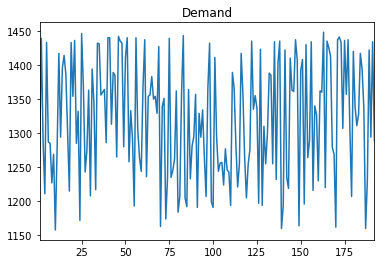
demand = Series(raw_demand, index = range(1, nb_periods+1))
# plot demand
demand.plot(title="Demand")
nb periods = 192
<matplotlib.axes._subplots.AxesSubplot at 0x23fbad3d588>
Step 4: Set up the prescriptive model
from docplex.mp.environment import Environment
env = Environment()
env.print_information()
* system is: Windows 64bit
* Python version 3.7.3, located at: c:\local\python373\python.exe
* docplex is present, version is (2, 11, 0)
* pandas is present, version is 0.25.1
Create the DOcplex model
The model contains all the business constraints and defines the objective.
from docplex.mp.model import Model

ucpm = Model("ucp")
Define the decision variables
Decision variables are:
The variable in_use[u,t] is 1 if and only if unit u is working at period t.
The variable turn_on[u,t] is 1 if and only if unit u is in production at period t.
The variable turn_off[u,t] is 1 if unit u is switched off at period t.
The variable production[u,t] is a continuous variables representing the production of energy for unit u at period t.
units = all_units
# periods range from 1 to nb_periods included
periods = range(1, nb_periods+1)

# in use[u,t] is true iff unit u is in production at period t
in_use = ucpm.binary_var_matrix(keys1=units, keys2=periods, name="in_use")

# true if unit u is turned on at period t
turn_on = ucpm.binary_var_matrix(keys1=units, keys2=periods, name="turn_on")

# true if unit u is switched off at period t
# modeled as a continuous 0-1 variable, more on this later
turn_off = ucpm.continuous_var_matrix(keys1=units, keys2=periods, lb=0, ub=1, name="turn_off")

# production of energy for unit u at period t
production = ucpm.continuous_var_matrix(keys1=units, keys2=periods, name="p")

# at this stage we have defined the decision variables.
ucpm.print_information()
Model: ucp
 - number of variables: 7680
   - binary=3840, integer=0, continuous=3840
 - number of constraints: 0
   - linear=0
 - parameters: defaults
 - problem type is: MILP
# Organize all decision variables in a DataFrame indexed by 'units' and 'periods'
df_decision_vars = DataFrame({'in_use': in_use, 'turn_on': turn_on, 'turn_off': turn_off, 'production': production})
# Set index names
df_decision_vars.index.names=['units', 'periods']

# Display first few rows of 'df_decision_vars' DataFrame
df_decision_vars.head()
| in_use | turn_on | turn_off | production | ||
|---|---|---|---|---|---|
| units | periods | ||||
| coal1 | 1 | in_use_coal1_1 | turn_on_coal1_1 | turn_off_coal1_1 | p_coal1_1 |
| 2 | in_use_coal1_2 | turn_on_coal1_2 | turn_off_coal1_2 | p_coal1_2 | |
| 3 | in_use_coal1_3 | turn_on_coal1_3 | turn_off_coal1_3 | p_coal1_3 | |
| 4 | in_use_coal1_4 | turn_on_coal1_4 | turn_off_coal1_4 | p_coal1_4 | |
| 5 | in_use_coal1_5 | turn_on_coal1_5 | turn_off_coal1_5 | p_coal1_5 |
Express the business constraints
Linking in-use status to production
Whenever the unit is in use, the production must be within the minimum and maximum generation.
# Create a join between 'df_decision_vars' and 'df_up' Data Frames based on common index id (ie: 'units')
# In 'df_up', one keeps only relevant columns: 'min_gen' and 'max_gen'
df_join_decision_vars_up = df_decision_vars.join(df_up[['min_gen', 'max_gen']], how='inner')

# Display first few rows of joined Data Frames
df_join_decision_vars_up.head()
| in_use | turn_on | turn_off | production | min_gen | max_gen | ||
|---|---|---|---|---|---|---|---|
| units | periods | ||||||
| coal1 | 1 | in_use_coal1_1 | turn_on_coal1_1 | turn_off_coal1_1 | p_coal1_1 | 100.0 | 425 |
| 2 | in_use_coal1_2 | turn_on_coal1_2 | turn_off_coal1_2 | p_coal1_2 | 100.0 | 425 | |
| 3 | in_use_coal1_3 | turn_on_coal1_3 | turn_off_coal1_3 | p_coal1_3 | 100.0 | 425 | |
| 4 | in_use_coal1_4 | turn_on_coal1_4 | turn_off_coal1_4 | p_coal1_4 | 100.0 | 425 | |
| 5 | in_use_coal1_5 | turn_on_coal1_5 | turn_off_coal1_5 | p_coal1_5 | 100.0 | 425 |
import pandas as pb
print(pd.__version__)
0.25.1
# When in use, the production level is constrained to be between min and max generation.
for item in df_join_decision_vars_up.itertuples(index=False):
    ucpm += (item.production <= item.max_gen * item.in_use)
    ucpm += (item.production >= item.min_gen * item.in_use)
Initial state
The solution must take into account the initial state. The initial state of use of the unit is determined by its initial production level.
# Initial state
# If initial production is nonzero, then period #1 is not a turn_on
# else turn_on equals in_use
# Dual logic is implemented for turn_off
for u in units:
    if df_up.initial[u] > 0:
        # if u is already running, not starting up
        ucpm.add_constraint(turn_on[u, 1] == 0)
        # turnoff iff not in use
        ucpm.add_constraint(turn_off[u, 1] + in_use[u, 1] == 1)
    else:
        # turn on at 1 iff in use at 1
        ucpm.add_constraint(turn_on[u, 1] == in_use[u, 1])
        # already off, not switched off at t==1
        ucpm.add_constraint(turn_off[u, 1] == 0)
ucpm.print_information()
Model: ucp
 - number of variables: 7680
   - binary=3840, integer=0, continuous=3840
 - number of constraints: 3860
   - linear=3860
 - parameters: defaults
 - problem type is: MILP
Ramp-up / ramp-down constraint
Variations of the production level over time in a unit is constrained by a ramp-up / ramp-down process.
We use the pandas groupby operation to collect all decision variables for each unit in separate series. Then, we iterate over units to post constraints enforcing the ramp-up / ramp-down process by setting upper bounds on the variation of the production level for consecutive periods.
# Use groupby operation to process each unit
for unit, r in df_decision_vars.groupby(level='units'):
    u_ramp_up = df_up.ramp_up[unit]
    u_ramp_down = df_up.ramp_down[unit]
    u_initial = df_up.initial[unit]
    # Initial ramp up/down
    # Note that r.production is a Series that can be indexed as an array (ie: first item index = 0)
    ucpm.add_constraint(r.production[0] - u_initial <= u_ramp_up)
    ucpm.add_constraint(u_initial - r.production[0] <= u_ramp_down)
    for (p_curr, p_next) in zip(r.production, r.production[1:]):
        ucpm.add_constraint(p_next - p_curr <= u_ramp_up)
        ucpm.add_constraint(p_curr - p_next <= u_ramp_down)

ucpm.print_information()
Model: ucp
 - number of variables: 7680
   - binary=3840, integer=0, continuous=3840
 - number of constraints: 7700
   - linear=7700
 - parameters: defaults
 - problem type is: MILP
Turn on / turn off
The following constraints determine when a unit is turned on or off.
We use the same pandas groupby operation as in the previous constraint to iterate over the sequence of decision variables for each unit.
# Turn_on, turn_off
# Use groupby operation to process each unit
for unit, r in df_decision_vars.groupby(level='units'):
    for (in_use_curr, in_use_next, turn_on_next, turn_off_next) in zip(r.in_use, r.in_use[1:], r.turn_on[1:], r.turn_off[1:]):
        # if unit is off at time t and on at time t+1, then it was turned on at time t+1
        ucpm.add_constraint(in_use_next - in_use_curr <= turn_on_next)

        # if unit is on at time t and time t+1, then it was not turned on at time t+1
        # mdl.add_constraint(in_use_next + in_use_curr + turn_on_next <= 2)

        # if unit is on at time t and off at time t+1, then it was turned off at time t+1
        ucpm.add_constraint(in_use_curr - in_use_next + turn_on_next == turn_off_next)
ucpm.print_information()
Model: ucp
 - number of variables: 7680
   - binary=3840, integer=0, continuous=3840
 - number of constraints: 11520
   - linear=11520
 - parameters: defaults
 - problem type is: MILP
Minimum uptime and downtime
When a unit is turned on, it cannot be turned off before a minimum uptime. Conversely, when a unit is turned off, it cannot be turned on again before a minimum downtime.
Again, let’s use the same pandas groupby operation to implement this constraint for each unit.
# Minimum uptime, downtime
for unit, r in df_decision_vars.groupby(level='units'):
    min_uptime   = df_up.min_uptime[unit]
    min_downtime = df_up.min_downtime[unit]
    # Note that r.turn_on and r.in_use are Series that can be indexed as arrays (ie: first item index = 0)
    for t in range(min_uptime, nb_periods):
        ctname = "min_up_{0!s}_{1}".format(*r.index[t])
        ucpm.add_constraint(ucpm.sum(r.turn_on[(t - min_uptime) + 1:t + 1]) <= r.in_use[t], ctname)

    for t in range(min_downtime, nb_periods):
        ctname = "min_down_{0!s}_{1}".format(*r.index[t])
        ucpm.add_constraint(ucpm.sum(r.turn_off[(t - min_downtime) + 1:t + 1]) <= 1 - r.in_use[t], ctname)
Demand constraint
Total production level must be equal or higher than demand on any period.
This time, the pandas operation groupby is performed on “periods” since we have to iterate over the list of all units for each period.
# Enforcing demand
# we use a >= here to be more robust,
# objective will ensure  we produce efficiently
for period, r in df_decision_vars.groupby(level='periods'):
    total_demand = demand[period]
    ctname = "ct_meet_demand_%d" % period
    ucpm.add_constraint(ucpm.sum(r.production) >= total_demand, ctname)
Express the objective
Operating the different units incur different costs: fixed cost, variable cost, startup cost, co2 cost.
In a first step, we define the objective as a non-weighted sum of all these costs.
The following pandas join operation groups all the data to calculate the objective in a single DataFrame.
# Create a join between 'df_decision_vars' and 'df_up' Data Frames based on common index ids (ie: 'units')
# In 'df_up', one keeps only relevant columns: 'fixed_cost', 'variable_cost', 'start_cost' and 'co2_cost'
df_join_obj = df_decision_vars.join(
    df_up[['fixed_cost', 'variable_cost', 'start_cost', 'co2_cost']], how='inner')

# Display first few rows of joined Data Frame
df_join_obj.head()
| in_use | turn_on | turn_off | production | fixed_cost | variable_cost | start_cost | co2_cost | ||
|---|---|---|---|---|---|---|---|---|---|
| units | periods | ||||||||
| coal1 | 1 | in_use_coal1_1 | turn_on_coal1_1 | turn_off_coal1_1 | p_coal1_1 | 208.61 | 22.536 | 5000 | 30 |
| 2 | in_use_coal1_2 | turn_on_coal1_2 | turn_off_coal1_2 | p_coal1_2 | 208.61 | 22.536 | 5000 | 30 | |
| 3 | in_use_coal1_3 | turn_on_coal1_3 | turn_off_coal1_3 | p_coal1_3 | 208.61 | 22.536 | 5000 | 30 | |
| 4 | in_use_coal1_4 | turn_on_coal1_4 | turn_off_coal1_4 | p_coal1_4 | 208.61 | 22.536 | 5000 | 30 | |
| 5 | in_use_coal1_5 | turn_on_coal1_5 | turn_off_coal1_5 | p_coal1_5 | 208.61 | 22.536 | 5000 | 30 |
# objective
total_fixed_cost = ucpm.sum(df_join_obj.in_use * df_join_obj.fixed_cost)
total_variable_cost = ucpm.sum(df_join_obj.production * df_join_obj.variable_cost)
total_startup_cost = ucpm.sum(df_join_obj.turn_on * df_join_obj.start_cost)
total_co2_cost = ucpm.sum(df_join_obj.production * df_join_obj.co2_cost)
total_economic_cost = total_fixed_cost + total_variable_cost + total_startup_cost

total_nb_used = ucpm.sum(df_decision_vars.in_use)
total_nb_starts = ucpm.sum(df_decision_vars.turn_on)

# store expression kpis to retrieve them later.
ucpm.add_kpi(total_fixed_cost   , "Total Fixed Cost")
ucpm.add_kpi(total_variable_cost, "Total Variable Cost")
ucpm.add_kpi(total_startup_cost , "Total Startup Cost")
ucpm.add_kpi(total_economic_cost, "Total Economic Cost")
ucpm.add_kpi(total_co2_cost     , "Total CO2 Cost")
ucpm.add_kpi(total_nb_used, "Total #used")
ucpm.add_kpi(total_nb_starts, "Total #starts")

# minimize sum of all costs
ucpm.minimize(total_fixed_cost + total_variable_cost + total_startup_cost + total_co2_cost)
Solve with Decision Optimization
If you’re using a Community Edition of CPLEX runtimes, depending on the size of the problem, the solve stage may fail and will need a paying subscription or product installation.
ucpm.print_information()
Model: ucp
 - number of variables: 7680
   - binary=3840, integer=0, continuous=3840
 - number of constraints: 15455
   - linear=15455
 - parameters: defaults
 - problem type is: MILP
assert ucpm.solve(), "!!! Solve of the model fails"
ucpm.report()
* model ucp solved with objective = 14213082.064
*  KPI: Total Fixed Cost    = 161025.131
*  KPI: Total Variable Cost = 8865900.433
*  KPI: Total Startup Cost  = 2832.000
*  KPI: Total Economic Cost = 9029757.564
*  KPI: Total CO2 Cost      = 5183324.500
*  KPI: Total #used         = 1335.000
*  KPI: Total #starts       = 3.000
Step 5: Investigate the solution and then run an example analysis
Now let’s store the results in a new pandas DataFrame.
For convenience, the different figures are organized into pivot tables with periods as row index and units as columns. The pandas unstack operation does this for us.
df_prods = df_decision_vars.production.apply(lambda v: v.solution_value).unstack(level='units')
df_used = df_decision_vars.in_use.apply(lambda v: v.solution_value).unstack(level='units')
df_started = df_decision_vars.turn_on.apply(lambda v: v.solution_value).unstack(level='units')

# Display the first few rows of the pivoted 'production' data
df_prods.head()
| units | coal1 | coal2 | diesel1 | diesel2 | diesel3 | diesel4 | gas1 | gas2 | gas3 | gas4 |
|---|---|---|---|---|---|---|---|---|---|---|
| periods | ||||||||||
| 1 | 425.0 | 215.0 | 90.0 | 87.0 | 0.0 | 0.0 | 109.4 | 52.0 | 165.0 | 115.6 |
| 2 | 425.0 | 365.0 | 90.0 | 87.0 | 0.0 | 0.0 | 78.0 | 71.0 | 165.0 | 158.0 |
| 3 | 425.0 | 312.0 | 90.0 | 87.0 | 0.0 | 0.0 | 0.0 | 52.0 | 165.0 | 158.0 |
| 4 | 425.0 | 234.0 | 90.0 | 87.0 | 0.0 | 0.0 | 0.0 | 52.0 | 165.0 | 158.0 |
| 5 | 425.0 | 365.0 | 90.0 | 87.0 | 0.0 | 0.0 | 0.0 | 143.0 | 165.0 | 158.0 |
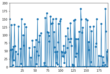
From these raw DataFrame results, we can compute derived results. For example, for a given unit and period, the reserve r(u,t) is defined as the unit’s maximum generation minus the current production.
df_spins = DataFrame(df_up.max_gen.to_dict(), index=periods) - df_prods

# Display the first few rows of the 'df_spins' Data Frame, representing the reserve for each unit, over time
df_spins.head()
| coal1 | coal2 | diesel1 | diesel2 | diesel3 | diesel4 | gas1 | gas2 | gas3 | gas4 | |
|---|---|---|---|---|---|---|---|---|---|---|
| 1 | 0.0 | 150.0 | 0.0 | 0.0 | 20.0 | 12.0 | 110.6 | 158.0 | 0.0 | 42.4 |
| 2 | 0.0 | 0.0 | 0.0 | 0.0 | 20.0 | 12.0 | 142.0 | 139.0 | 0.0 | 0.0 |
| 3 | 0.0 | 53.0 | 0.0 | 0.0 | 20.0 | 12.0 | 220.0 | 158.0 | 0.0 | 0.0 |
| 4 | 0.0 | 131.0 | 0.0 | 0.0 | 20.0 | 12.0 | 220.0 | 158.0 | 0.0 | 0.0 |
| 5 | 0.0 | 0.0 | 0.0 | 0.0 | 20.0 | 12.0 | 220.0 | 67.0 | 0.0 | 0.0 |
Let’s plot the evolution of the reserves for the “coal2” unit:
df_spins.coal2.plot(style='o-', ylim=[0,200])
<matplotlib.axes._subplots.AxesSubplot at 0x23fd903bf60>
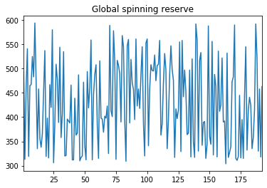
Now we want to sum all unit reserves to compute the global spinning reserve. We need to sum all columns of the DataFrame to get an aggregated time series. We use the pandas sum method with axis=1 (for rows).
global_spin = df_spins.sum(axis=1)
global_spin.plot(title="Global spinning reserve")
<matplotlib.axes._subplots.AxesSubplot at 0x23fda312710>
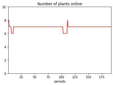
Number of plants online by period
The total number of plants online at each period t is the sum of in_use variables for all units at this period. Again, we use the pandas sum with axis=1 (for rows) to sum over all units.
df_used.sum(axis=1).plot(title="Number of plants online", kind='line', style="r-", ylim=[0, len(units)])
<matplotlib.axes._subplots.AxesSubplot at 0x23fda37f9b0>
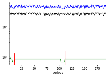
Costs by period
# extract unit cost data
all_costs = ["fixed_cost", "variable_cost", "start_cost", "co2_cost"]
df_costs = df_up[all_costs]

running_cost = df_used * df_costs.fixed_cost
startup_cost = df_started * df_costs.start_cost
variable_cost = df_prods * df_costs.variable_cost
co2_cost = df_prods * df_costs.co2_cost
total_cost = running_cost + startup_cost + variable_cost + co2_cost

running_cost.sum(axis=1).plot(style='g')
startup_cost.sum(axis=1).plot(style='r')
variable_cost.sum(axis=1).plot(style='b',logy=True)
co2_cost.sum(axis=1).plot(style='k')
<matplotlib.axes._subplots.AxesSubplot at 0x23fda3c7e80>
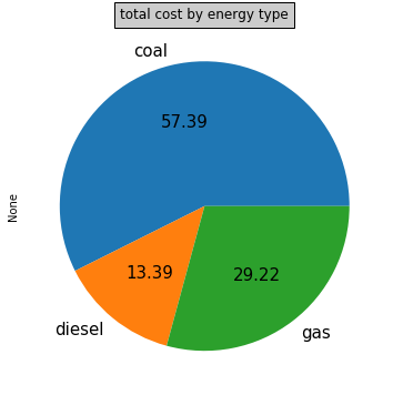
Cost breakdown by unit and by energy
# Calculate sum by column (by default, axis = 0) to get total cost for each unit
cost_by_unit = total_cost.sum()

# Create a dictionary storing energy type for each unit, from the corresponding pandas Series
unit_energies = df_up.energy.to_dict()

# Group cost by unit type and plot total cost by energy type in a pie chart
gb = cost_by_unit.groupby(unit_energies)
# gb.sum().plot(kind='pie')
gb.sum().plot.pie(figsize=(6, 6),autopct='%.2f',fontsize=15)

plt.title('total cost by energy type', bbox={'facecolor':'0.8', 'pad':5})
Text(0.5, 1.0, 'total cost by energy type')
Arbitration between CO2 cost and economic cost
Economic cost and CO2 cost usually push in opposite directions. In the above discussion, we have minimized the raw sum of economic cost and CO2 cost, without weights. But how good could we be on CO2, regardless of economic constraints? To know this, let’s solve again with CO2 cost as the only objective.
# first retrieve the co2 and economic kpis
co2_kpi = ucpm.kpi_by_name("co2") # does a name matching
eco_kpi = ucpm.kpi_by_name("eco")
prev_co2_cost = co2_kpi.compute()
prev_eco_cost = eco_kpi.compute()
print("* current CO2 cost is: {}".format(prev_co2_cost))
print("* current $$$ cost is: {}".format(prev_eco_cost))
# now set the objective
old_objective = ucpm.objective_expr # save it
ucpm.minimize(co2_kpi.as_expression())
* current CO2 cost is: 5183324.5
* current $$$ cost is: 9029757.56390015
assert ucpm.solve(), "Solve failed"
min_co2_cost = ucpm.objective_value
min_co2_eco_cost = eco_kpi.compute()
print("* absolute minimum for CO2 cost is {}".format(min_co2_cost))
print("* at this point $$$ cost is {}".format(min_co2_eco_cost))
* absolute minimum for CO2 cost is 3399032.0
* at this point $$$ cost is 12434227.620000225
As expected, we get a significantly lower CO2 cost when minimized alone, at the price of a higher economic cost.
We could do a similar analysis for economic cost to estimate the absolute minimum of the economic cost, regardless of CO2 cost.
# minimize only economic cost
ucpm.minimize(eco_kpi.as_expression())
assert ucpm.solve(), "Solve failed"
min_eco_cost = ucpm.objective_value
min_eco_co2_cost = co2_kpi.compute()
print("* absolute minimum for $$$ cost is {}".format(min_eco_cost))
print("* at this point CO2 cost is {}".format(min_eco_co2_cost))
* absolute minimum for $$$ cost is 8887433.859000005
* at this point CO2 cost is 5375417.0
Again, the absolute minimum for economic cost is lower than the figure we obtained in the original model where we minimized the sum of economic and CO2 costs, but here we significantly increase the CO2.
But what happens in between these two extreme points?
To investigate, we will divide the interval of CO2 cost values in smaller intervals, add an upper limit on CO2, and minimize economic cost with this constraint. This will give us a Pareto optimal point with at most this CO2 value.
To avoid adding many constraints, we add only one constraint with an extra variable, and we change only the upper bound of this CO2 limit variable between successive solves.
Then we iterate (with a fixed number of iterations) and collect the cost values.
# add extra variable
co2_limit = ucpm.continuous_var(lb=0)
# add a named constraint which limits total co2 cost to this variable:
max_co2_ctname = "ct_max_co2"
co2_ct = ucpm.add_constraint(co2_kpi.as_expression() <= co2_limit, max_co2_ctname)
co2min = min_co2_cost
co2max = min_eco_co2_cost
def explore_ucp(nb_iters, eps=1e-5):

    step = (co2max-co2min)/float(nb_iters)
    co2_ubs = [co2min + k * step for k in range(nb_iters+1)]

    # ensure we minimize eco
    ucpm.minimize(eco_kpi.as_expression())
    all_co2s = []
    all_ecos = []
    for k in range(nb_iters+1):
        co2_ub = co2min + k * step
        print(" iteration #{0} co2_ub={1}".format(k, co2_ub))
        co2_limit.ub = co2_ub + eps
        assert ucpm.solve() is not None, "Solve failed"
        cur_co2 = co2_kpi.compute()
        cur_eco = eco_kpi.compute()
        all_co2s.append(cur_co2)
        all_ecos.append(cur_eco)
    return all_co2s, all_ecos
#explore the co2/eco frontier in 50 points
co2s, ecos = explore_ucp(nb_iters=50)
iteration #0 co2_ub=3399032.0
iteration #1 co2_ub=3438559.7
iteration #2 co2_ub=3478087.4
iteration #3 co2_ub=3517615.1
iteration #4 co2_ub=3557142.8
iteration #5 co2_ub=3596670.5
iteration #6 co2_ub=3636198.2
iteration #7 co2_ub=3675725.9
iteration #8 co2_ub=3715253.6
iteration #9 co2_ub=3754781.3
iteration #10 co2_ub=3794309.0
iteration #11 co2_ub=3833836.7
iteration #12 co2_ub=3873364.4
iteration #13 co2_ub=3912892.1
iteration #14 co2_ub=3952419.8
iteration #15 co2_ub=3991947.5
iteration #16 co2_ub=4031475.2
iteration #17 co2_ub=4071002.9
iteration #18 co2_ub=4110530.6
iteration #19 co2_ub=4150058.3
iteration #20 co2_ub=4189586.0
iteration #21 co2_ub=4229113.7
iteration #22 co2_ub=4268641.4
iteration #23 co2_ub=4308169.1
iteration #24 co2_ub=4347696.8
iteration #25 co2_ub=4387224.5
iteration #26 co2_ub=4426752.2
iteration #27 co2_ub=4466279.9
iteration #28 co2_ub=4505807.6
iteration #29 co2_ub=4545335.3
iteration #30 co2_ub=4584863.0
iteration #31 co2_ub=4624390.7
iteration #32 co2_ub=4663918.4
iteration #33 co2_ub=4703446.1
iteration #34 co2_ub=4742973.8
iteration #35 co2_ub=4782501.5
iteration #36 co2_ub=4822029.2
iteration #37 co2_ub=4861556.9
iteration #38 co2_ub=4901084.6
iteration #39 co2_ub=4940612.3
iteration #40 co2_ub=4980140.0
iteration #41 co2_ub=5019667.7
iteration #42 co2_ub=5059195.4
iteration #43 co2_ub=5098723.1
iteration #44 co2_ub=5138250.8
iteration #45 co2_ub=5177778.5
iteration #46 co2_ub=5217306.2
iteration #47 co2_ub=5256833.9
iteration #48 co2_ub=5296361.6
iteration #49 co2_ub=5335889.3
iteration #50 co2_ub=5375417.0
# normalize all values by dividing by their maximum
eco_max = min_co2_eco_cost
nxs = [c / co2max for c in co2s]
nys = [e / eco_max for e in ecos]
# plot a scatter chart of x=co2, y=costs
plt.scatter(nxs, nys)
# plot as one point
plt.plot(prev_co2_cost/co2max, prev_eco_cost/eco_max, "rH", markersize=16)
plt.xlabel("co2 cost")
plt.ylabel("economic cost")
plt.show()
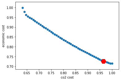
This figure demonstrates that the result obtained in the initial model clearly favored economic cost over CO2 cost: CO2 cost is well above 95% of its maximum value.
Summary
You learned how to set up and use IBM Decision Optimization CPLEX Modeling for Python to formulate a Mathematical Programming model and solve it with IBM Decision Optimization on Cloud.
References
Need help with DOcplex or to report a bug? Please go here.
Contact us at IBM Community.
Copyright � 2017-2019 IBM. IPLA licensed Sample Materials.